Prepare datasets

Three-way datasets are stored as tensors (three-dimensional arrays). However, both methods support two ways of providing the data - natural (as a 3-way array) as well as unfolded into a 2-way matrix (rows are samples and columns are column-wise unfolded sample matrices).

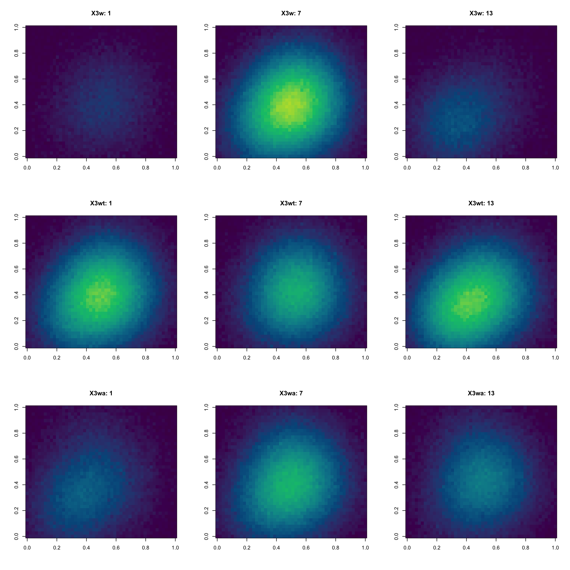
This tutorial is based on simulated 3-way data, the simulation was done similarly to what is described in 10.1021/acs.analchem.3c05096. Target samples contain two components in random concentrations. Alternative class samples contain the same two components + a third component in random concentrations. The component instrumental profiles are partially overlapped Gaussian functions, defined in 40 and 50 channels in each data mode (hence the data matrices have \(50\times40\) dimension). Gaussian noise was then added to all signals at a level of 10% with respect to the mean signal. The author is grateful to Alejandro Olivieri for sharing a MATLAB script implementing simulations and helping with the tutorial.

You can load the data by running:

library(mdatools)

data(data3w)
print(str(data3w))

## List of 3
##  $ X3w : num [1:80, 1:50, 1:40] 0.012 0.03 0.0228 0.0437 0.0353 ...
##  $ X3wt: num [1:20, 1:50, 1:40] 0.02798 0.00561 0.03457 0.03881 0.02374 ...
##  $ X3wa: num [1:60, 1:50, 1:40] 0.0249 0.01478 0.03083 0.01011 0.00696 ...
## NULL

As we can see, all datasets are represented in the form of 3-way arrays, the training set, X3w, contains 80 samples, the test target setX3wt, contains 20 samples and the test alternative set, X3wa, contains 60 samples. The dimensions of each sample matrix are 50 x 40.

Let’s visualize some of them in the form of heatmaps.

col <- hcl.colors(256, "Viridis")

par(mfrow = c(3, 3))
for (n in names(data3w)) {
   X = data3w[[n]]
   X[X < 0] = 0
   for (i in c(1, 7, 13)) {
      image(X[i, , ], main = sprintf("%s: %d", n, i),
         zlim = c(0, 0.35), useRaster = TRUE, col = col)
   }
}

As mentioned above, it is not necessary to reshape three-way data. However, we will create a reshaped array for the training set just to demonstrate that the methods work on both representations. In addition to that we will also generate vectors with reference class labels.

data(data3w)

# attach the list, so we can use "X3w" instead of "data3w$X3w"
attach(data3w)

## The following object is masked _by_ .GlobalEnv:
## 
##     X3w

## The following objects are masked from data3w (pos = 3):
## 
##     X3w, X3wa, X3wt

## The following objects are masked from data3w (pos = 5):
## 
##     X3w, X3wa, X3wt

# prepare unfolded 2-way data for training set plus generate the class labels
X2w <- X3w
dim(X2w) <- c(dim(X3w)[1], prod(dim(X3w)[2:3]))
c.train <- rep("target", nrow(X2w))

# generate class labels for target and alternative class samples in test set
c.test.target <- rep("target", dim(X3wt)[1])
c.test.alt <- rep("alt", dim(X3wa)[1])

# combine the target and alternative class samples into a single test set
nt <- dim(X3wt)[1]
na <- dim(X3wa)[1]
n <- nt + na
c.test <- c(c.test.target, c.test.alt)
X3wb <- array(0, dim = c(n, dim(X3wt)[2], dim(X3wt)[3]))
X3wb[1:nt, , ] <- X3wt
X3wb[(nt + 1):n, , ] <- X3wa