Calibration and validation
The model calibration is similar to PCA, but there are several additional arguments, which are important for classification. First of all, it is a class name, which is a second mandatory argument. The class name is a string, which can be used later e.g. for identifying class members for testing.
You can also provide significance level for extreme objects, alpha, and significance level for detection of outliers, gamma. By default \(0.05\) (5%) and \(0.01\) (1%) will be used. These two parameters can be also adjusted later without rebuilding the whole model.
By default DD-SIMCA model computes critical limits and does all classification using two types of estimator: "classic" (sometimes also referred by "moments") and "robust". The robust estimator should be used for detection of outliers, while the final model should use the classic one. You do not need to preselect the type of the limits, any plot and any outcomes can be shown for both types of limits by providing argument limType as it will be shown below.
To run all examples you need to download dataset Oregano from web-application: here is a direct link: https://mda.tools/ddsimca/Oregano.zip. Download and unzip it to the same folder where you plan to keep your R code. In my case all data files are collected inside Oregano folder.
Let’s load the training set first and prepare it for the model:
library(mdatools)

dc <- read.csv("./Oregano/Target_Train.csv", row.names = 1, check.names = FALSE)
show(dc[1:5, 1:5])
## Class 8998.367 8990.654 8982.939 8975.226
## Bio01 Oregano -1.036600 -1.036965 -1.034487 -1.032063
## Bio02 Oregano -1.040406 -1.035694 -1.035552 -1.035854
## Bio03 Oregano -1.042949 -1.041892 -1.039863 -1.041063
## Bio04 Oregano -1.052614 -1.050210 -1.050617 -1.052789
## Bio05 Oregano -1.034859 -1.032732 -1.033896 -1.032058As you can see, the first column, Class, contains the class labels, which we do not need for training (we need to know the label though). The other columns contain values of NIR spectra of Oregano samples, already preprocessed. The column names are wavenumbers in reciprocal centimeters, let’s take them and assign as xaxis-values:
xc = as.matrix(dc[, -1])
w = as.numeric(colnames(xc))
attr(xc, "xaxis.values") = w
attr(xc, "xaxis.name") = expression("Wavenumbers, cm"^{-1})

mdaplot(xc, type = "l", main = "Oregano training set")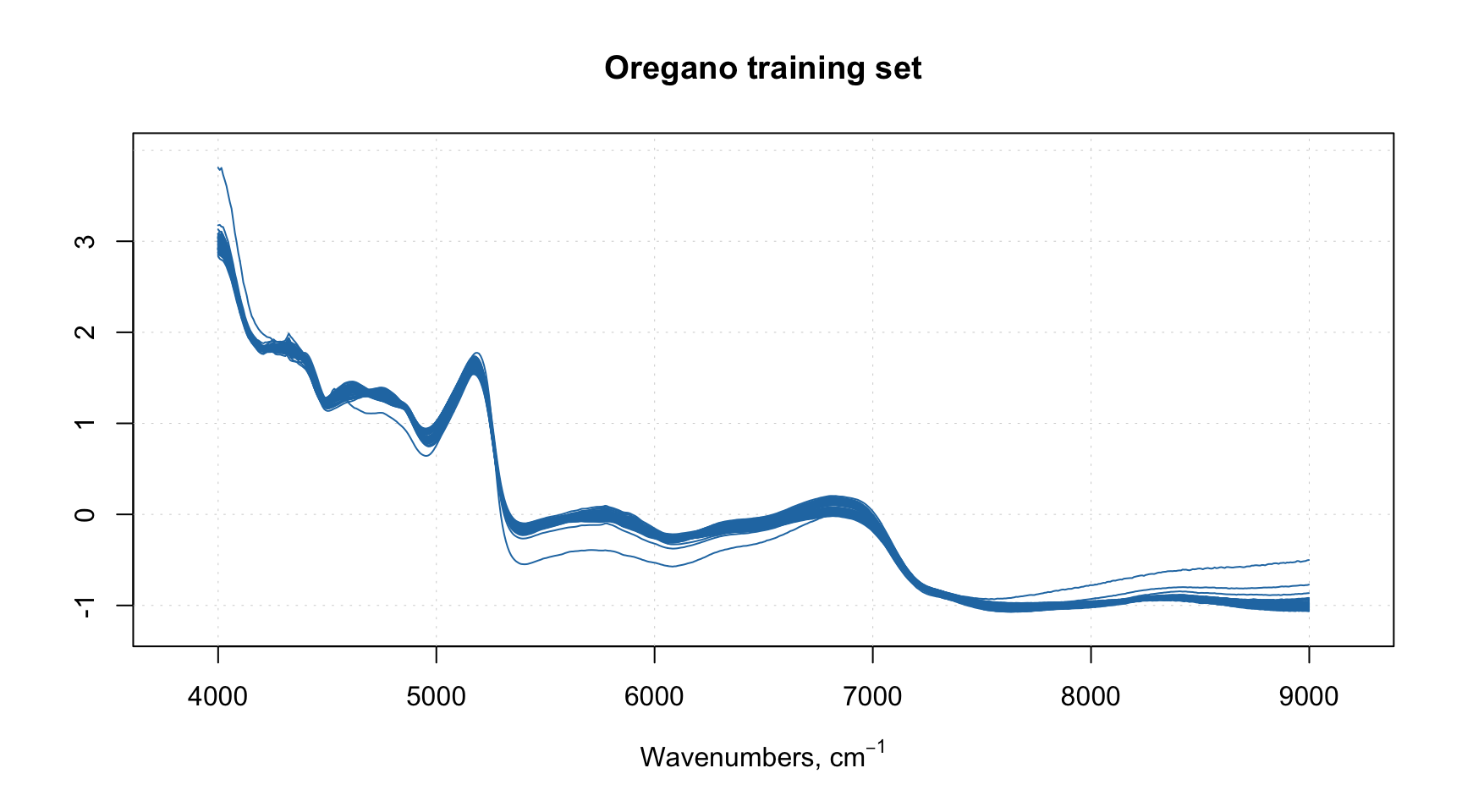
We can notice one or two spectra which behave differently, we will discuss them later.
Now we can train the model:
##
## DD-SIMCA model for class 'Oregano'
##
## Number of components: 10
## Number of selected components: 10
## Type of limits: classic
## Alpha: 0.05
## Gamma: 0.01
##
##     Expvar Cumexpvar In Out TP FN   Sens
## Cal 0.1458     99.61 50   2 50  2 0.9615
## Pv  1.3179     98.64 32  20 32 20 0.6154
As you may notice, we provided value for argument pcv. These are parameters for Procrustes cross-validation, which was introduced in the PCA chapter. Here, instead of creating the PV-set manually, DD-SIMCA does everything itself. As one can see, the model with \(A = 10\) components performs badly on PV-set with sensitivity of \(0.6154\).
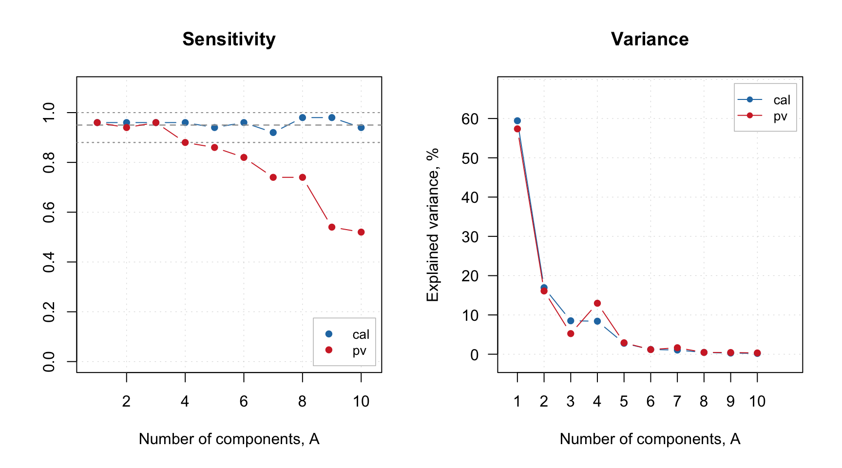
Let’s start with looking at the Sensitivity plot and the PC variance:
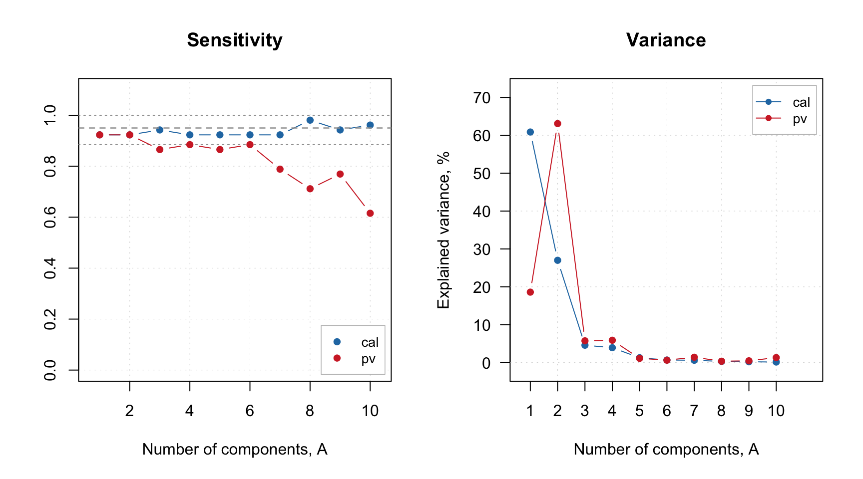
The parameter show.ci for sensitivity plot adds 95% confidence interval for the expected sensitivity which is computed based on the significance level and the size of the dataset. The dashed point in the middle shows the expected value and the two dotted lines — the boundaries of the interval.
As one can see, the sensitivity for PV-set (red color) is within the interval for the first two PCs, and then falling apart. After \(A = 6\) the overfitting becomes obvious. The variance plot shows a large discrepancy between the individual variance values for training and PV-sets which possibly indicates the presence of outliers.
The next code shows Acceptance plot for \(A = 2\). This plot is similar to PCA’s Distance plot; however, in this case the objects are also color coded according to their role (regular, extreme or outlier). The plot can be shown using robust and classic estimators. The code in fact reproduces two top plots from the Figure 2 of the paper.
par(mfrow = c(1, 2))
plotAcceptance(m, ncomp = 2, show.labels = TRUE)
plotAcceptance(m, ncomp = 2, limType = "robust", show.labels = TRUE)
As you can see, the plot is made for calibration set. If you want to make it for PV-set, either specify parameter res or simply make it for the result object:
par(mfrow = c(1, 2))
plotAcceptance(m, res = "pv", ncomp = 2, show.labels = TRUE)
plotAcceptance(m$res$pv, ncomp = 2, show.labels = TRUE)
Anyway, on both sets of plots, Drg12 is clearly an outlier. Let’s remove it and re-create the model. There are two possibilities, either you can remove it from the original dataset or just provide the name of the sample to the model using exclrows parameter. Let’s try the second option:
m = ddsimca(xc, "Oregano", ncomp = 10, pcv = list("ven", 4), exclrows = c("Drg12"))

par(mfrow = c(1, 2))
plotAcceptance(m, ncomp = 2, show.labels = TRUE)
plotAcceptance(m, ncomp = 2, limType = "robust", show.labels = TRUE)
Apparently the object Drg13 is an outlier as well, let’s exclude it:
m = ddsimca(xc, "Oregano", ncomp = 10, pcv = list("ven", 4), exclrows = c("Drg12", "Drg13"))

par(mfrow = c(1, 2))
plotAcceptance(m, ncomp = 2, show.labels = TRUE)
plotAcceptance(m, ncomp = 2, limType = "robust", show.labels = TRUE)
Now both classic and robust estimators show a decent picture without outliers. You can also show the plots using log-transformed distances:
par(mfrow = c(1, 2))
plotAcceptance(m, ncomp = 2, log = TRUE, show.labels = TRUE)
plotAcceptance(m, ncomp = 2, log = TRUE, limType = "robust", show.labels = TRUE)
Before we proceed with figure of merits and optimization of number of components, let’s look at the spectra of the removed objects to confirm their different behaviour:
par(mfrow = c(1, 1))
mdaplot(xc, type = "l", col = "gray", main = "Training set spectra")
mdaplot(mda.subset(xc, c("Drg12", "Drg13")), type = "l", col = "red", show.axes = FALSE)
Apparently they indeed look like outliers.
Now let’s check at the sensitivity and variance again:
Now the variance of training and PV-set looks similar and the sensitivity plot points at \(A = 3\) as the optimal number of components. Let’s set this parameter for the model and check the summary:
##
## DD-SIMCA model for class 'Oregano'
##
## Excluded rows: 2
## Number of components: 10
## Number of selected components: 3
## Type of limits: classic
## Alpha: 0.05
## Gamma: 0.01
##
##     Expvar Cumexpvar In Out TP FN Sens
## Cal  8.512     84.88 48   4 48  2 0.96
## Pv   5.248     78.72 48   2 48  2 0.96
If you for any reason want to change significance level for the model, you can do it as follows:
##
## DD-SIMCA model for class 'Oregano'
##
## Excluded rows: 2
## Number of components: 10
## Number of selected components: 3
## Type of limits: classic
## Alpha: 0.01
## Gamma: 0.001
##
##     Expvar Cumexpvar In Out TP FN Sens
## Cal  8.512     84.88 49   3 49  1 0.98
## Pv   5.248     78.72 49   1 49  1 0.98
As you can see, the results and the figures of merit for training set and PV-set are recomputed automatically. In the code above, we saved the modified model to a separate variable, so we can continue with default parameters.
Since DD-SIMCA model is also a PCA model, you can show all plots relevant for PCA:

And of course you can look at the Extremes plot to check for possible overfitting:
The same applies to the results object.
par(mfrow = c(1, 2))
plotScores(m$res$cal, show.labels = TRUE)
plotVariance(m$res$cal, type = "h", show.labels = TRUE)