Additional methods and features

This section describes additional methods for data preprocessing. They work similar to any other method, the only difference is that they do not work with the prep, prep.fit, prep.apply methods. Just use them separately.

Element-wise transformations

Function prep.transform() allows you to apply an element-wise transformation — when the same transformation function is being applied to each element (each value) of the data matrix. This can be used, for example, in case of regression, when it is necessary to apply transformations which remove a non-linear relationship between predictors and responses.

Often such a transformation is either logarithmic or a power transformation. We can of course just apply a built-in R function e.g. log() or sqrt(), however in this case all additional attributes will be dropped in the preprocessed data. In order to tackle this and, also, to give the possibility of combining different preprocessing methods together, you can use a function prep.transform() for this purpose.

The syntax of the function is as follows: prep.transform(data, fun, ...), where data is a matrix with the original data values, you want to preprocess (transform), fun is a reference to transformation function and ... are optional additional arguments for the function. You can provide either one of the R functions, which are element-wise (meaning the function is being applied to each element of a matrix), such as log, exp, sqrt, etc. or define your own function.

Here is an example:

# create a matrix with 3 variables (skewed random values)
X <- cbind(
   exp(rnorm(100, 5, 1)),
   exp(rnorm(100, 5, 1)) + 100 ,
   exp(rnorm(100, 5, 1)) + 200
)

# apply log transformation using built in "log" function
Y1 <- prep.transform(X, log)

# apply power transformation using manual function with additional argument
Y2 <- prep.transform(X, function(x, p) x^p, p = 0.2)

# show boxplots for the original and the transformed data
par(mfrow = c(1,3))
boxplot(X, main = "Original values")
boxplot(Y1, main = "Preprocessed (log)")
boxplot(Y2, main = "Preprocessed (power)")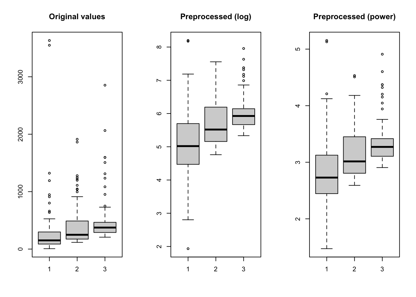

As already mentioned, the prep.transform() preserves all additional attributes, e.g. names and values for axes, excluded columns or rows, etc. Here is another example demonstrating this:

# generate two curves using sin() and cos() and add some attributes
t <- (-31:31)/10
X <- rbind(sin(t), cos(t))
rownames(X) <- c("s1", "s2")

# we make x-axis values as time, which span a range from 0 to 620 seconds
attr(X, "xaxis.name") <- "Time, s"
attr(X, "xaxis.values") <- (t * 10 + 31) * 10
attr(X, "name") <- "Time series"

# transform the dataset using squared transformation
Y <- prep.transform(X, function(x) x^2)

# show plots for the original and the transformed data
par(mfrow = c(2, 1))
mdaplotg(X, type = "l")
mdaplotg(Y, type = "l")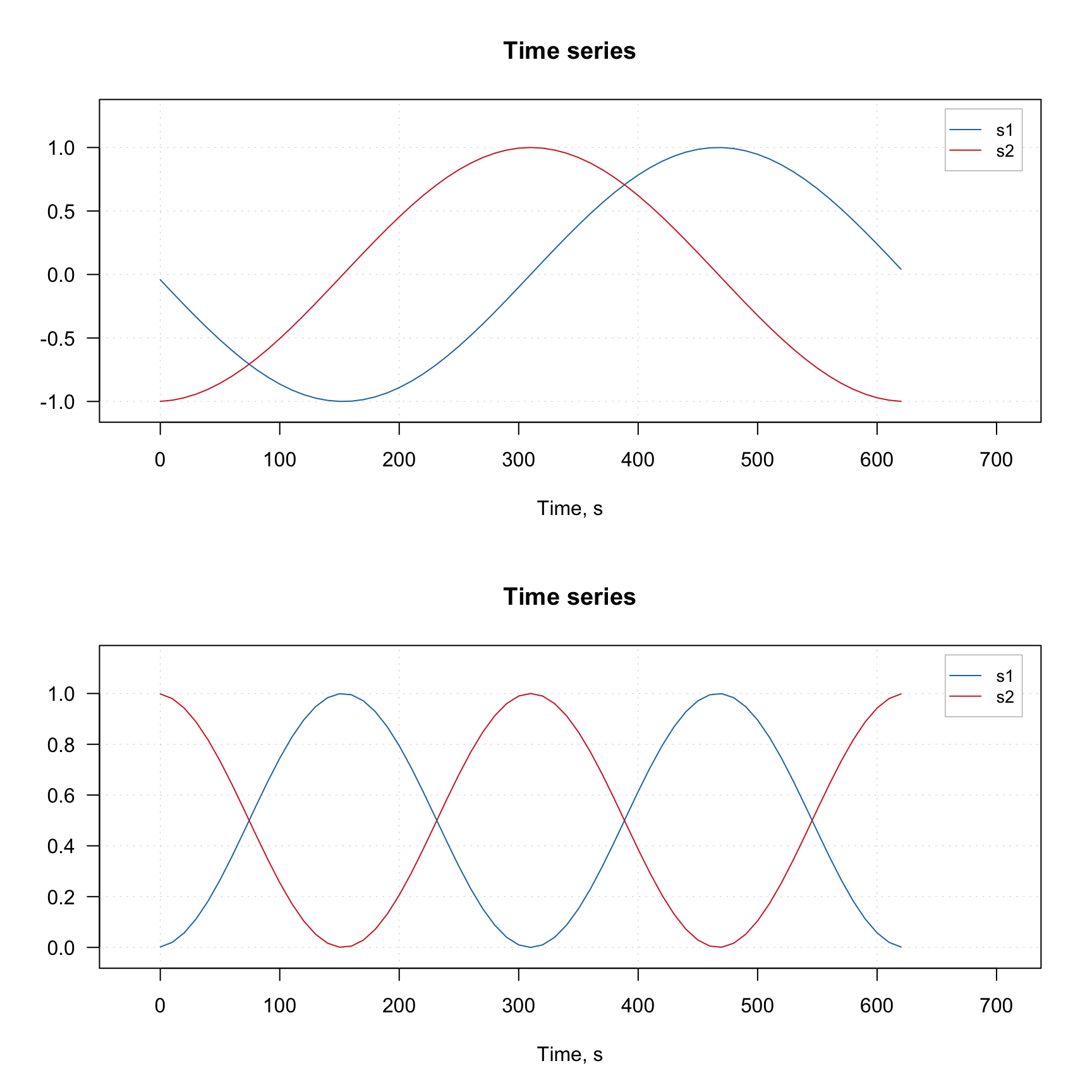

Notice that the x-axis values for the original and the transformed data (which we defined using corresponding attribute) are the same.

Kubelka-Munk transformation

Kubelka-Munk is a useful preprocessing method for diffuse reflection spectra (e.g. taken for powders or rough surface). It transforms the reflectance spectra R to K/M units as follows: \((1 - R)^2 / 2R\).

The method is implemented as prep.ref2km(X), where X is a matrix with non-negative reflectance values.

Replacing missing values

This is not directly a preprocessing method, but can be considered as such. This method allows one to replace missing values in your dataset with the approximated ones.

The method uses PCA based approach described in this paper. The main idea is that we fit the dataset with a PCA model (e.g. PCA NIPALS algorithm can work even if the data contains missing values) and then approximate the missing values as if they were lying in the PC space.

The method has the same parameters as any PCA model. However, instead of specifying number of components you must specify another parameter, expvarlim, which specifies the portion of variance the model must explain. The default value is 0.95 which corresponds to 95% of the explained variance. You can also specify if data must be centered (default TRUE) and scaled/standardized (default FALSE). See more details by running ?pca.mvreplace.

The example below shows a trivial case. First we generate a simple dataset. Then we replace some of the numbers with missing values (NA) and then apply the method to approximate them.

library(mdatools)

# generate a matrix with correlated variables
s = 1:6
odata = cbind(s, 2*s, 4*s)

# add some noise and labels for columns and rows
set.seed(42)
odata = odata + matrix(rnorm(length(odata), 0, 0.1), dim(odata))
colnames(odata) = paste0("X", 1:3)
rownames(odata) = paste0("O", 1:6)

# make a matrix with missing values
mdata = odata
mdata[5, 2] = mdata[2, 3] = NA

# replace missing values with approximated
rdata = pca.mvreplace(mdata, scale = TRUE)

# show all matrices together
show(round(cbind(odata, mdata, round(rdata, 2)), 3))

##       X1     X2     X3    X1     X2     X3   X1    X2    X3
## O1 1.137  2.151  3.861 1.137  2.151  3.861 1.14  2.15  3.86
## O2 1.944  3.991  7.972 1.944  3.991     NA 1.94  3.99  7.51
## O3 3.036  6.202 11.987 3.036  6.202 11.987 3.04  6.20 11.99
## O4 4.063  7.994 16.064 4.063  7.994 16.064 4.06  7.99 16.06
## O5 5.040 10.130 19.972 5.040     NA 19.972 5.04 10.21 19.97
## O6 5.989 12.229 23.734 5.989 12.229 23.734 5.99 12.23 23.73

# show the difference between original and approximated values
show(round(odata - rdata, 3))

##    X1     X2    X3
## O1  0  0.000 0.000
## O2  0  0.000 0.465
## O3  0  0.000 0.000
## O4  0  0.000 0.000
## O5  0 -0.076 0.000
## O6  0  0.000 0.000

As you can see, the method guessed that the two missing values must be 7.51 and 10.21, while the original values were 7.97 and 10.13.

The method works if the total number of missing values does not exceed 20% (10% if the dataset is small).