Multiclass classification

Several SIMCA models can be combined to a special object simcam, which is used to make a multiclass classification. Besides this, it also allows calculating distance between individual models and a discrimination power — importance of variables to discriminate between any two classes. Let’s see how it works.

First we create three single-class SIMCA models with individual settings, such as number of optimal components and alpha.

m.set = simca(X.set, "setosa", 3, alpha = 0.01)
m.set = selectCompNum(m.set, 1)

m.vir = simca(X.vir, "virginica", 3)
m.vir = selectCompNum(m.vir, 2)

m.ver = simca(X.ver, "versicolor", 3)
m.ver = selectCompNum(m.ver, 1)

Then we combine the models into a simcam model object. Summary will show the performance on calibration set, which is a combination of calibration sets for each of the individual models

mm = simcam(list(m.set, m.vir, m.ver))
summary(mm)

## 
## SIMCA multiple classes classification (class simcam)
## 
## Number of classes: 3
## Info: 
## 
## Summary for calibration results
##            Ncomp TP FP TN FN Spec. Sens. Accuracy
## setosa         1 25  0 50  0  1.00  1.00     1.00
## virginica      2 22  3 47  3  0.94  0.88     0.92
## versicolor     1 25  3 47  0  0.94  1.00     0.96

Now we apply the combined model to the test set and look at the predictions.

res = predict(mm, Xt, ct)
plotPredictions(res)

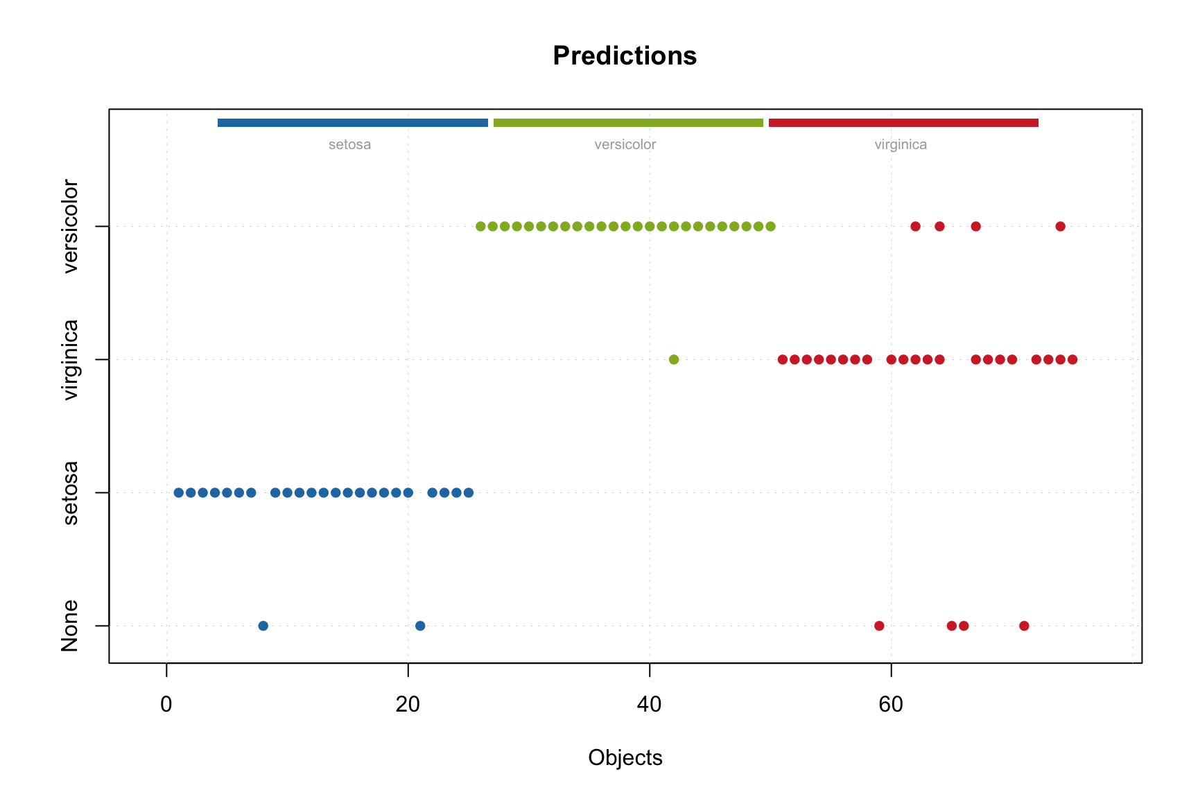
In this case, the predictions are shown only for the number of components each model found optimal. The names of classes along y-axis are the individual models. Similarly we can show the predicted values.

show(res$c.pred[20:30, 1, ])

##    setosa virginica versicolor
## 40      1        -1         -1
## 42     -1        -1         -1
## 44      1        -1         -1
## 46      1        -1         -1
## 48      1        -1         -1
## 50      1        -1         -1
## 52     -1        -1          1
## 54     -1        -1          1
## 56     -1        -1          1
## 58     -1        -1          1
## 60     -1        -1          1

Method getConfusionMatrix() is also available in this case.

show(getConfusionMatrix(res))

##            setosa virginica versicolor None
## setosa         23         0          0    2
## virginica       0        21          4    4
## versicolor      0         1         25    0

There are three additional plots available for multiclass SIMCA model. First of all it is a distance between a selected model and the others.

par(mfrow = c(1, 2))
plotModelDistance(mm, 1)
plotModelDistance(mm, 2)

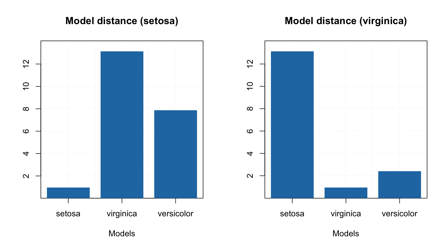The plot shows not a real distance but rather a similarity between a selected model and the others as a ratio of residual variances. You can find more detailed description about how model is calculated in description of the method or in help for plotModelDistance.simcam function.

The second plot is a discrimination power, mentioned in the beginning of the section.

par(mfrow = c(1, 2))
plotDiscriminationPower(mm, c(1, 3), show.labels = TRUE)
plotDiscriminationPower(mm, c(2, 3), show.labels = TRUE)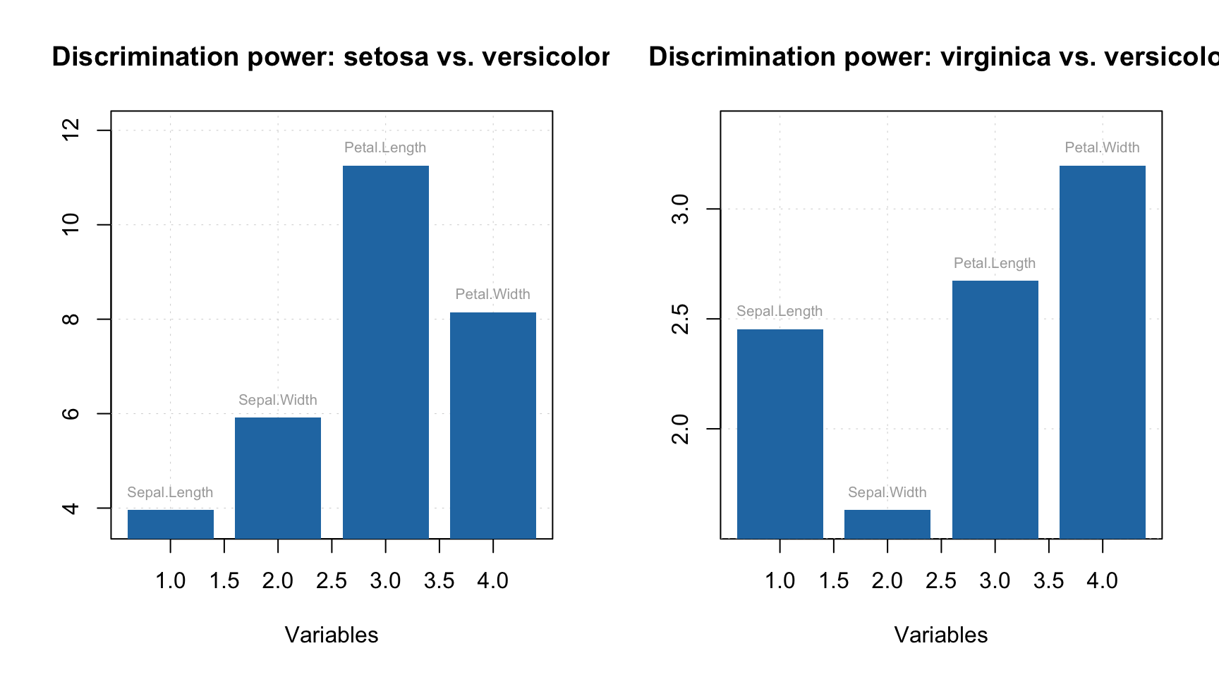

And, finally, a Cooman’s plot showing an orthogonal distance, \(q\), from objects to two selected classes/models.

par(mfrow = c(1, 2))
plotCooman(mm, c(1, 3), show.labels = TRUE)
plotCooman(mm, c(2, 3), show.labels = TRUE)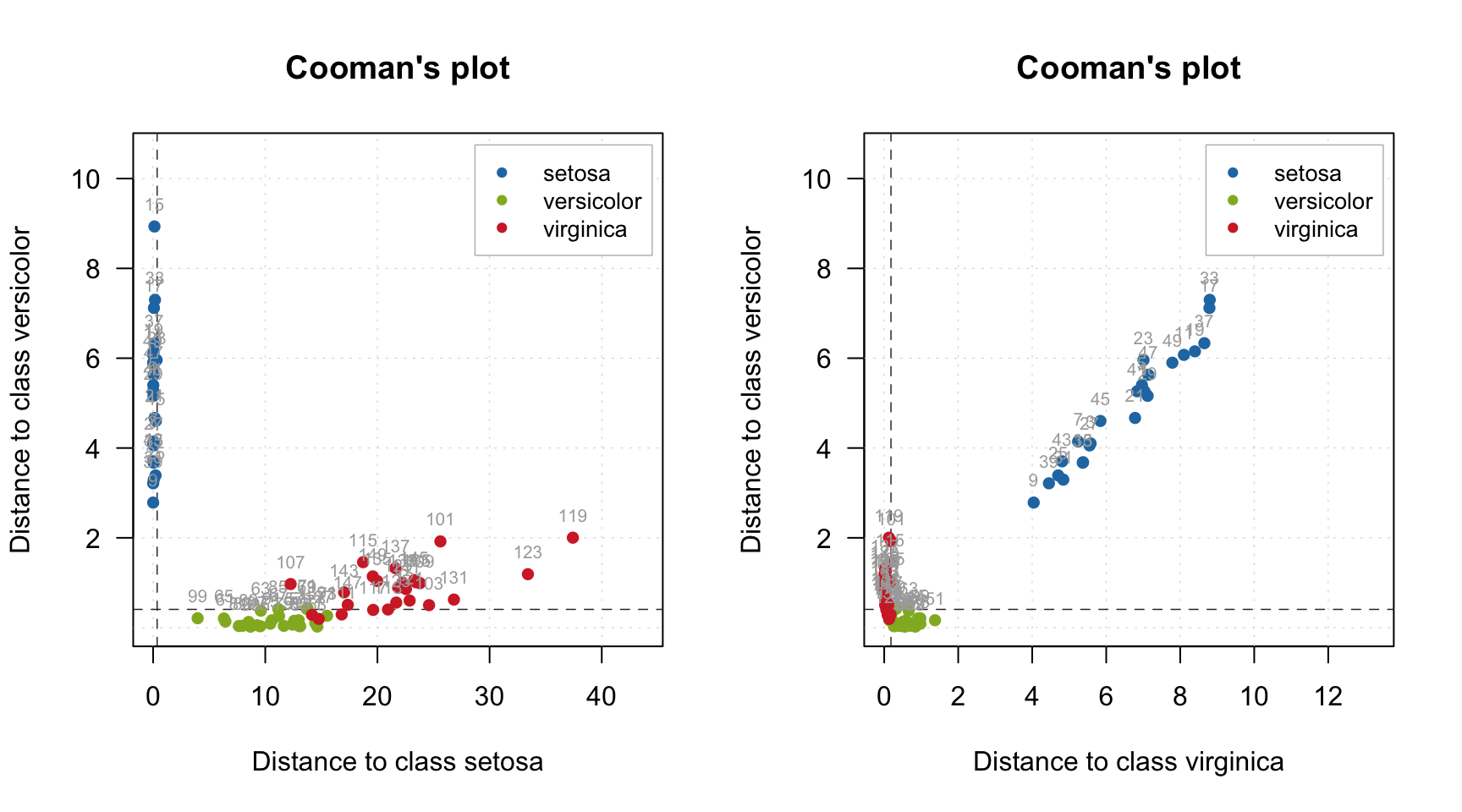

The limits, shown as dashed lines, are computed using chi-square distribution but only for \(q\) values.