Combining methods together
All methods mentioned above (there are more, which are discussed later in this section) can be combined into a preprocessing chain, which is just an R object (list). After that this chain can be “trained” (for example if methods have parameters that depend on training set, like centering, scaling or EMSC) and be applied as a whole to any dataset. You can also provide such a list of preprocessing methods as parameters for most of the models.
It can be handy if you need to apply the same chain of methods to different datasets, so you can combine them once, train their parameters and use it as many times as needed. In this section we discuss how to do this.
First of all, you can see the list of the preprocessing methods available for this feature as well as all necessary information about them if you run prep.list() as shown below:
##
##
## List of available preprocessing methods:
##
##
##  Select user-defined variables (columns of dataset).
##  ---------------
##  name: 'varsel'
##  parameters:
##   'var.ind': indices of variables (columns) to select.
##
##
##  Normalization.
##  ---------------
##  name: 'norm'
##  parameters:
##   'type': type of normalization ('area', 'sum', 'length', 'is', 'snv', 'pqn').
##   'col.ind': indices of columns (variables) for normalization to internal standard peak.
##   'ref.spectrum': reference spectrum for PQN normalization.
##
##
##  Savitzky-Golay filter.
##  ---------------
##  name: 'savgol'
##  parameters:
##   'width': width of the filter.
##   'porder': polynomial order.
##   'dorder': derivative order.
##
##
##  Asymmetric least squares baseline correction.
##  ---------------
##  name: 'alsbasecorr'
##  parameters:
##   'plambda': power of the penalty parameter (e.g. if plambda = 5, lambda = 10^5)
##   'p': asymmetry ratio (should be between 0 and 1)
##   'max.niter': maximum number of iterations
##
##
##  Removes cosmic spikes.
##  ---------------
##  name: 'spikes'
##  parameters:
##   'width': width of the moving median filter
##   'threshold': threshold for spike detection
##
##
##  Center dataset columns.
##  ---------------
##  name: 'center'
##  parameters:
##   'type': what to use for centering ('mean', or 'median')
##
##
##  Scale dataset columns.
##  ---------------
##  name: 'scale'
##  parameters:
##   'type': what to use for scaling ('sd', 'iqr', 'range', or 'pareto')
##
##
##  Multiplicative scatter correction.
##  ---------------
##  name: 'emsc'
##  parameters:
##   'degree': polynomial degree (0 for MSC)
##   'mspectrum': reference spectrum (if NULL mean spectrum will be used).
What you need to know is the name of the method and which parameters you can or want to provide (if you do not specify any parameters, default values will be used instead).
Let’s start with a simple example, where we want to take spectra from Simdata, and, first of all, apply Savitzky-Golay with filter width = 5, polynomial degree = 2 and derivative order = 1. Then we want to normalize them using SNV and get rid of all spectral values from 300 nm and above. Here is how to make a preprocessing object for this sequence:
data(simdata)
w <- simdata$wavelength

myprep <- list(
   prep("savgol", width = 5, porder = 2, dorder = 1),
   prep("norm", type = "snv"),
   prep("varsel", var.ind = w < 300)
)
Now you can apply the whole sequence to any spectral data by using function prep.apply():
Xc <- simdata$spectra.c
attr(Xc, "xaxis.values") <- w
attr(Xc, "xaxis.name") <- "Wavelength, nm"

Xcp <- prep.apply(myprep, Xc)

par(mfrow = c(2, 1))
mdaplot(Xc, type = "l", xlim = c(200, 350), main = "Raw spectra")
mdaplot(Xcp, type = "l", xlim = c(200, 350), main = "Preprocessed spectra")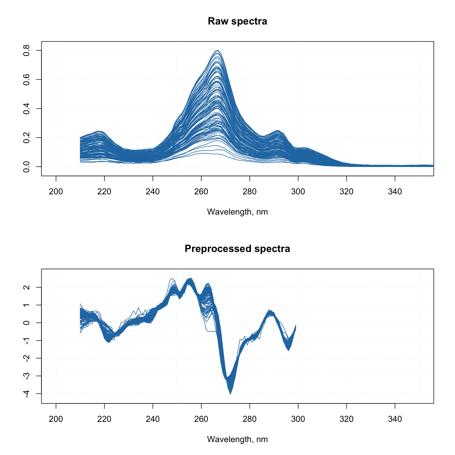
Now let’s consider another example, where we have a calibration set and a test set. We need to create preprocessing sequence for the calibration set and, let’s say, we ended up with the following sequence:
- Smoothing with linear Savitzky-Golay filter (
width = 9) - MSC correction (EMSC with
degree = 0) - Normalization to unit area
- Removing the part with wavelength > 300 nm
- Mean centering
We have an issue here. Both centering and EMSC methods require additional parameters which are computed based on the training set. EMSC needs mean spectrum, which will be used as a reference. And centering needs values for centering. This issue can be solved by using method prep.fit():
# define calibration and test sets
Xc <- simdata$spectra.c
Xt <- simdata$spectra.t
w <- simdata$wavelength
attr(Xt, "xaxis.values") <- attr(Xc, "xaxis.values") <- w
attr(Xt, "xaxis.name") <- attr(Xc, "xaxis.name") <- "Wavelength, nm"

# create a sequence of preprocessing methods
myprep <- list(
   prep("savgol", width = 9, porder = 1),
   prep("emsc", degree = 0),
   prep("norm", type = "area"),
   prep("varsel", var.ind = w < 300),
   prep("center")
)

# fit the preprocessing model - will estimate all needed parameters based on Xc
myprep <- prep.fit(myprep, Xc)

# apply the fitted model to both sets
Xcp <- prep.apply(myprep, Xc)
Xtp <- prep.apply(myprep, Xt)

par(mfrow = c(2, 2))
mdaplot(Xc, type = "l", main = "Calibration set, raw")
mdaplot(Xt, type = "l", main = "Test set, raw")
mdaplot(Xcp, type = "l", main = "Calibration set, preprocessed")
mdaplot(Xtp, type = "l", main = "Test set, preprocessed")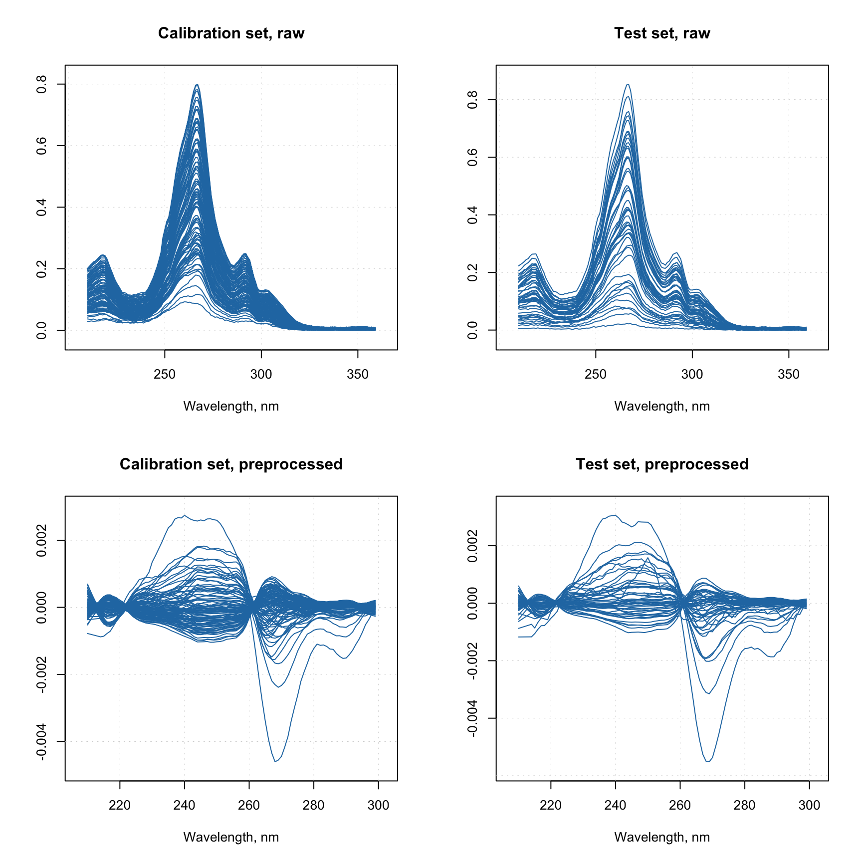
The fitted preprocessing model can be saved to an RData file as any other R object.