Variable selection
PLS allows one to calculate several statistics, which can be used to select most important (or remove least important) variables in order to improve performance and make model simpler. The first two are VIP-scores (variables important for projection) and Selectivity ratio. All details and theory can be found e.g. here.
Both parameters can be shown as plots and as vector of values for a selected y-variable. Take into account that when you make a plot for VIP scores or Selectivity ratio, the corresponding values should be computed first, which can take some time for large datasets.
Here is an example of corresponding plots.
par(mfrow = c(2, 2))
plotVIPScores(m)
plotVIPScores(m, ncomp = 2, type = "h", show.labels = TRUE)
plotSelectivityRatio(m)
plotSelectivityRatio(m, ncomp = 2, type = "h", show.labels = TRUE)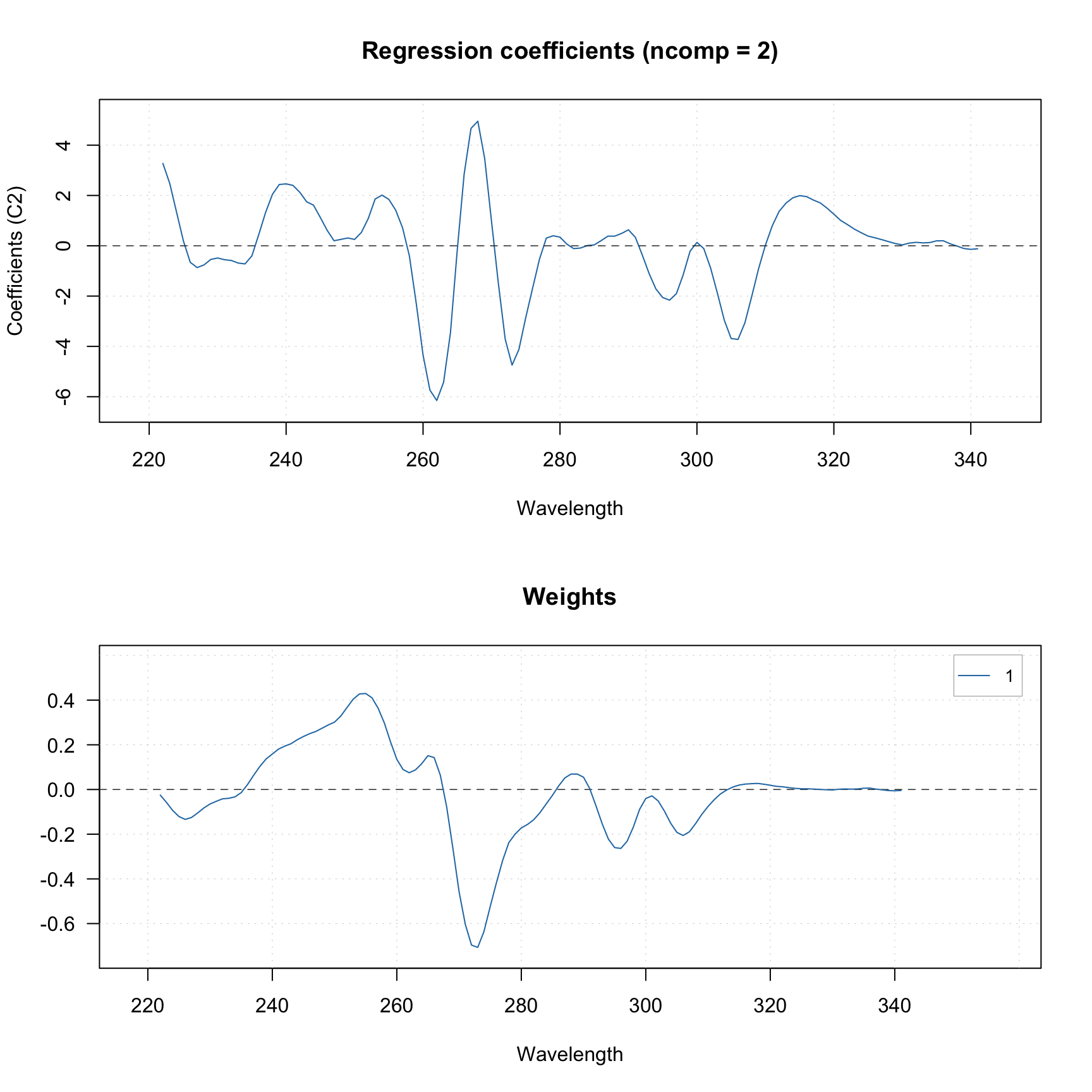
To compute the values without plotting use vipscores() and selratio() functions. In the example below, I create two other PLS models by excluding variables with VIP score or selectivity ratio below a threshold (I use 0.5 and 2 correspondingly) and show the performance for both.
vip = vipscores(m, ncomp = 2)
m2 = pls(Xc, yc, 4, scale = T, cv = 1, exclcols = (vip < 0.5))
summary(m2)
##
## PLS model (class pls) summary
## -------------------------------
## Info:
## Number of selected components: 2
## Cross-validation: full (leave one out)
## Excluded columns: 4
##
## Response variable: Shoesize
## X cumexpvar Y cumexpvar R2 RMSE Slope Bias RPD
## Cal 89.80722 95.27241 0.953 0.842 0.953 0.0000 4.70
## Cv NA NA 0.933 1.005 0.935 0.0254 3.94##
## PLS model (class pls) summary
## -------------------------------
## Info:
## Number of selected components: 2
## Cross-validation: full (leave one out)
## Excluded columns: 6
##
## Response variable: Shoesize
## X cumexpvar Y cumexpvar R2 RMSE Slope Bias RPD
## Cal 98.77528 95.79889 0.958 0.794 0.958 0.000 4.98
## Cv NA NA 0.946 0.903 0.944 0.014 4.38Another way is to make an inference about regression coefficients and calculate confidence intervals and p-values for each variable. This can be done using Jack-Knife approach, when model is cross-validated using a sufficient number of segments (at least ten) and statistics are calculated using the distribution of regression coefficient values obtained for each step. The statistics are automatically computed when you use full cross-validation.
The statistics are calculated for each y-variable and each available number of components. When you show a plot for regression coefficients, you can show the confidence intervals by using parameter show.ci = TRUE as shown in examples below.
par(mfrow = c(2, 2))
plotRegcoeffs(mjk, type = "h", show.ci = TRUE, show.labels = TRUE)
plotRegcoeffs(mjk, ncomp = 2, type = "h", show.ci = TRUE, show.labels = TRUE)
plotRegcoeffs(mjk, type = "l", show.ci = TRUE, show.labels = TRUE)
plotRegcoeffs(mjk, ncomp = 2, type = "l", show.ci = TRUE, show.labels = TRUE)
Calling function summary() for regression coefficients allows to get all calculated statistics.
##
## Regression coefficients for Shoesize (ncomp = 2)
## ------------------------------------------------
##               Coeffs   Std. err. t-value p-value        2.5%       97.5%
## Height    0.19357436 0.008270469   23.39   0.000  0.17646559  0.21068313
## Weight    0.18935489 0.005386414   35.12   0.000  0.17821224  0.20049754
## Hairleng -0.17730737 0.010368912  -17.09   0.000 -0.19875710 -0.15585764
## Age       0.02508113 0.026525148    0.95   0.351 -0.02979032  0.07995258
## Income    0.01291497 0.033491494    0.39   0.702 -0.05636746  0.08219740
## Beer      0.11441573 0.017851922    6.40   0.000  0.07748621  0.15134524
## Wine      0.08278735 0.030960265    2.68   0.013  0.01874117  0.14683354
## Sex      -0.17730737 0.010368912  -17.09   0.000 -0.19875710 -0.15585764
## Swim      0.19426871 0.013654151   14.21   0.000  0.16602295  0.22251448
## Region    0.02673161 0.023989628    1.12   0.275 -0.02289471  0.07635794
## IQ       -0.01705852 0.032399035   -0.53   0.602 -0.08408103  0.04996399
##
## Degrees of freedom (Jack-Knifing): 23##
## Regression coefficients for Shoesize (ncomp = 2)
## ------------------------------------------------
## Coeffs Std. err. t-value p-value 0.5% 99.5%
## Height 0.19357436 0.008270469 23.39 0.000 0.170356376 0.21679234
## Weight 0.18935489 0.005386414 35.12 0.000 0.174233417 0.20447636
## Hairleng -0.17730737 0.010368912 -17.09 0.000 -0.206416384 -0.14819835
## Age 0.02508113 0.026525148 0.95 0.351 -0.049383866 0.09954612
## Income 0.01291497 0.033491494 0.39 0.702 -0.081106896 0.10693683
## Beer 0.11441573 0.017851922 6.40 0.000 0.064299387 0.16453206
## Wine 0.08278735 0.030960265 2.68 0.013 -0.004128502 0.16970321
## Sex -0.17730737 0.010368912 -17.09 0.000 -0.206416384 -0.14819835
## Swim 0.19426871 0.013654151 14.21 0.000 0.155936928 0.23260050
## Region 0.02673161 0.023989628 1.12 0.275 -0.040615325 0.09407855
## IQ -0.01705852 0.032399035 -0.53 0.602 -0.108013488 0.07389645
##
## Degrees of freedom (Jack-Knifing): 23Function getRegcoeffs() in this case may also return corresponding t-value, standard error, p-value, and confidence interval for each of the coefficient (except intercept) if the user specifies a parameter full. The standard error and confidence intervals are also computed for raw, non-standardized, variables (similar to coefficients).
##               Estimated    Std. err.     t-value      p-value          2.5%
## Intercept  1.342626e+01           NA          NA           NA            NA
## Height     7.456695e-02 3.185875e-03  23.3854388 0.000000e+00  0.0679764667
## Weight     4.896328e-02 1.392816e-03  35.1242970 0.000000e+00  0.0460820210
## Hairleng  -6.865495e-01 4.014933e-02 -17.0926429 1.443290e-14 -0.7696047104
## Age        1.081716e-02 1.143995e-02   0.9524214 3.507861e-01 -0.0128481769
## Income     5.642220e-06 1.463158e-05   0.3875343 7.019238e-01 -0.0000246255
## Beer       5.010542e-03 7.817789e-04   6.3971862 1.579903e-06  0.0033933089
## Wine       7.511377e-03 2.809055e-03   2.6802915 1.336266e-02  0.0017004042
## Sex       -6.865495e-01 4.014933e-02 -17.0926429 1.443290e-14 -0.7696047104
## Swim       1.010496e-01 7.102257e-03  14.2147650 7.018830e-13  0.0863574493
## Region     1.035071e-01 9.288992e-02   1.1174095 2.753561e-01 -0.0886503166
## IQ        -5.277164e-03 1.002285e-02  -0.5285419 6.021868e-01 -0.0260110098
##                   97.5%
## Intercept            NA
## Height     8.115743e-02
## Weight     5.184454e-02
## Hairleng  -6.034943e-01
## Age        3.448250e-02
## Income     3.590994e-05
## Beer       6.627775e-03
## Wine       1.332235e-02
## Sex       -6.034943e-01
## Swim       1.157417e-01
## Region     2.956646e-01
## IQ         1.545668e-02
## attr(,"name")
## [1] "Regression coefficients for  Shoesize"
It is also possible to change significance level for confidence intervals.
##               Estimated    Std. err.     t-value      p-value          0.5%
## Intercept  1.342626e+01           NA          NA           NA            NA
## Height     7.456695e-02 3.185875e-03  23.3854388 0.000000e+00  6.562313e-02
## Weight     4.896328e-02 1.392816e-03  35.1242970 0.000000e+00  4.505318e-02
## Hairleng  -6.865495e-01 4.014933e-02 -17.0926429 1.443290e-14 -7.992621e-01
## Age        1.081716e-02 1.143995e-02   0.9524214 3.507861e-01 -2.129862e-02
## Income     5.642220e-06 1.463158e-05   0.3875343 7.019238e-01 -3.543353e-05
## Beer       5.010542e-03 7.817789e-04   6.3971862 1.579903e-06  2.815826e-03
## Wine       7.511377e-03 2.809055e-03   2.6802915 1.336266e-02 -3.745830e-04
## Sex       -6.865495e-01 4.014933e-02 -17.0926429 1.443290e-14 -7.992621e-01
## Swim       1.010496e-01 7.102257e-03  14.2147650 7.018830e-13  8.111117e-02
## Region     1.035071e-01 9.288992e-02   1.1174095 2.753561e-01 -1.572661e-01
## IQ        -5.277164e-03 1.002285e-02  -0.5285419 6.021868e-01 -3.341467e-02
##                   99.5%
## Intercept            NA
## Height     8.351077e-02
## Weight     5.287338e-02
## Hairleng  -5.738369e-01
## Age        4.293295e-02
## Income     4.671797e-05
## Beer       7.205258e-03
## Wine       1.539734e-02
## Sex       -5.738369e-01
## Swim       1.209880e-01
## Region     3.642803e-01
## IQ         2.286034e-02
## attr(,"name")
## [1] "Regression coefficients for  Shoesize"
The p-values, t-values and standard errors are stored each as a 3-way array similar to regression coefficients. The selection can be made by comparing e.g. p-values with a threshold similar to what we have done with VIP-scores and selectivity ratio.
##   Height   Weight Hairleng      Age   Income     Beer     Wine      Sex
##    FALSE    FALSE    FALSE     TRUE     TRUE    FALSE    FALSE    FALSE
##     Swim   Region       IQ
##    FALSE     TRUE     TRUE
Here p.values[, 2, 1] means values for all predictors, model with two components, first y-variable.
##
## PLS model (class pls) summary
## -------------------------------
## Info:
## Number of selected components: 3
## Cross-validation: full (leave one out)
## Excluded columns: 4
##
## Response variable: Shoesize
##     X cumexpvar Y cumexpvar    R2  RMSE Slope    Bias  RPD
## Cal    97.85476    97.79127 0.978 0.575 0.978  0.0000 6.87
## Cv NA NA 0.965 0.727 0.972 -0.0161 5.44## Estimated
## Intercept 4.952691046
## Height 0.091079963
## Weight 0.052708955
## Hairleng -0.315927643
## Age 0.000000000
## Income 0.000000000
## Beer 0.009320427
## Wine 0.018524717
## Sex -0.315927643
## Swim 0.134354170
## Region 0.000000000
## IQ 0.000000000
## attr(,"exclrows")
## Age Income Region IQ
## 4 5 10 11
## attr(,"name")
## [1] "Regression coefficients for Shoesize"As you can see, the variables Age, Income, Region and IQ have been excluded as they are not related to the Shoesize, which seems to be correct.
Variable selection as well as all described above can be also carried out for PLS discriminant analysis (PLS-DA), which will be explained later in one of the next chapters.