Distances and critical limits

As it was written in the brief theoretical section about PCA, when data objects are being projected to a principal component space, two distances are calculated and stored as a part of PCA results (pcares object). The first is a squared orthogonal Euclidean distance from original position of an object to the PC space, also known as orthogonal distance and denoted as Q or q. The distance shows how well the object is fitted by the PCA model and allows one to detect objects that do not follow a common trend, captured by the PCs.

The second distance shows how far a projection of an object to the PC space is from the origin. This distance is also known as the Hotelling T² distance or the score distance, which is also denoted as h-distance. To compute the h-distance, scores should first be normalized by dividing them by the corresponding singular values (or eigenvalues if we deal with squared scores). The h-distance allows to see extreme objects — which are far from the origin.

In previous versions of the mdatools method plotDistances() was known as plotResiduals(). It is still available for compatibility but if you write a new code, use plotDistances() instead.

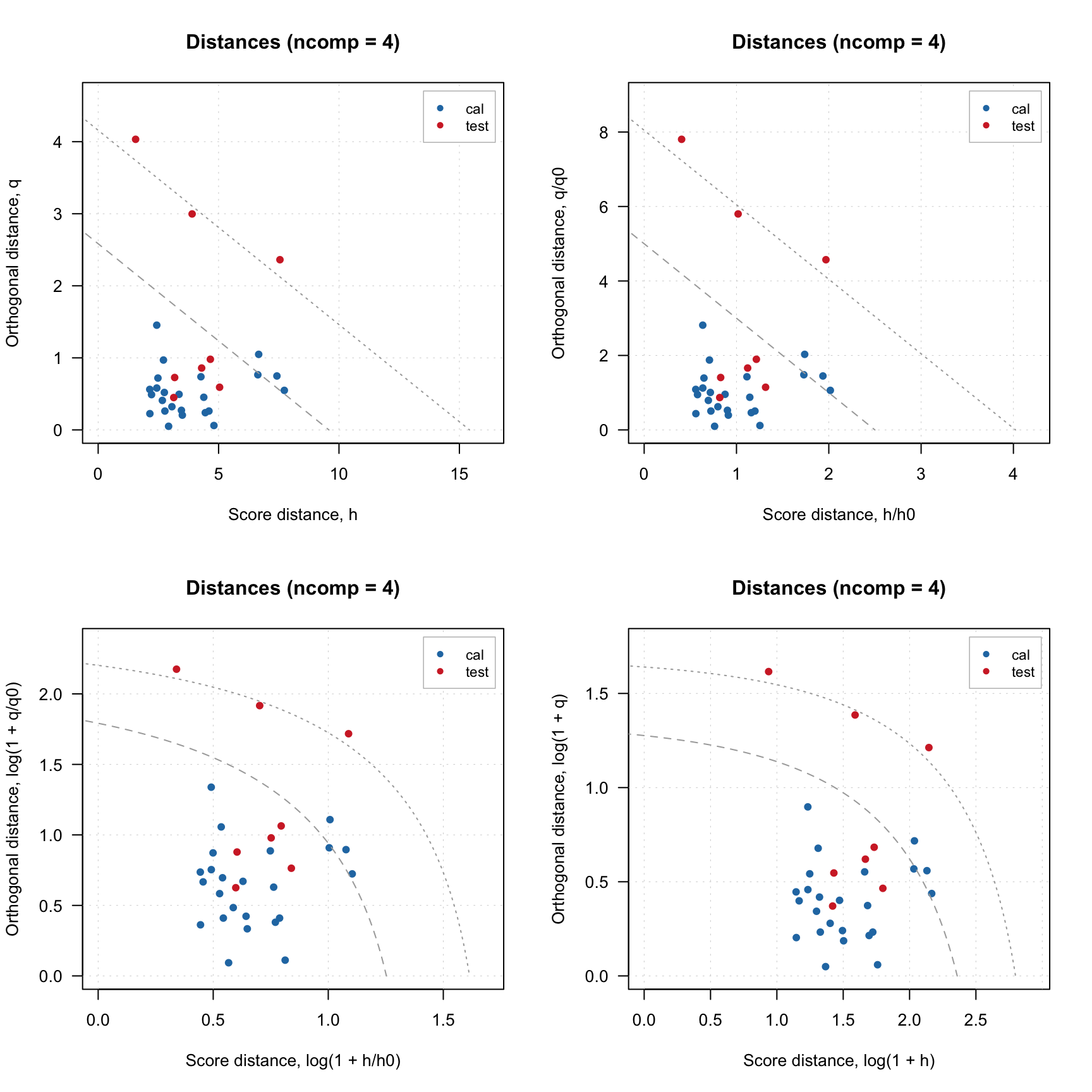
In mdatools both distances are calculated for all objects in dataset and all possible components. So every distance is represented by \(I \times A\) matrix (will remind here that \(I\) is the number of objects or rows in data matrix and \(A\) is number of components in PCA model), the first column contains distances for a model with only one component, second — for model with two components, and so on. The distances can be visualized using method plotDistances() which is available both for PCA results as well as for PCA model. In the case of model the plot shows distances both for calibration set and test set (if available).

Here is an example, where I split People data to calibration and test set as in one of the examples in previous sections and show distance plot for model and result objects.

data(people)

# split People data by taking every 4th measurement to a test set
idx = seq(4, 32, 4)
Xc = people[-idx, ]
Xt = people[idx, ]

# train PCA model with test set validation
m = pca(Xc, 4, scale = TRUE, x.test = Xt)

# show the results
par(mfrow = c(2, 2))
plotDistances(m, main = "Distances for model")
plotDistances(m, ncomp = 2, main = "Distances for model (2 PCs)")
plotDistances(m$res$cal, main = "Distances for calibration set")
plotDistances(m$res$test, main = "Distances for test set")

As it was briefly mentioned before, if residual/distance plot is made for a model, it also shows two critical limits: the dashed line is a limit for extreme objects and the dotted line is a limit for outliers. The position of the lines is defined by significance levels, alpha and gamma. For example, if alpha = 0.05, it is expected that 5% of the training samples will be beyond the critical limit for extreme objects (dashed line). Parameter gamma is a similar parameter for outlier detection, it defines the position of the dotted line (any object beyond this line is considered as outlier).

They are computed as critical limits using chi-square distribution, which approximates the distribution of the distance values. More details can be found in this paper.

If you want to hide them, just use additional parameter show.limits = FALSE. You can also change the color, line type and width for the lines by using options lim.col, lim.lty and lim.lwd as it is shown below.

par(mfrow = c(1, 2))
plotDistances(m, show.limits = FALSE)
plotDistances(m, lim.col = c("red", "orange"), lim.lwd = c(2, 2), lim.lty = c(1, 2))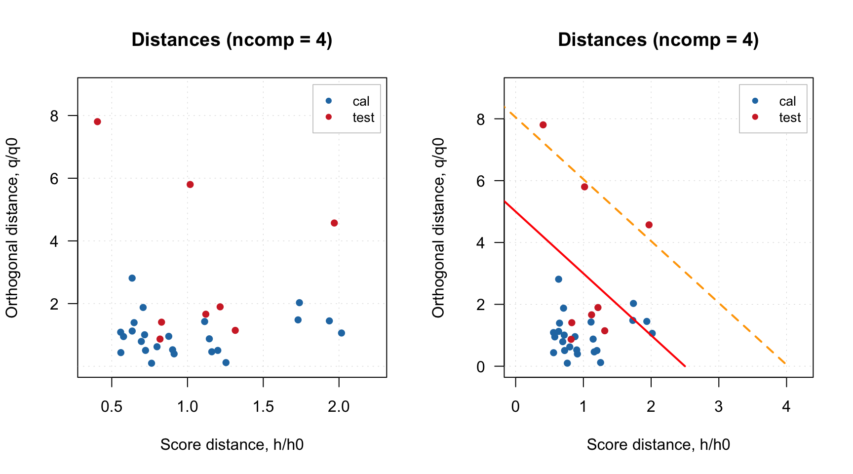

It is necessary to provide a vector with two values for each argument (first for extreme objects and second for outliers border).

Finally, you can also notice that for model plot the distance values are normalized (\(h/h_0\) and \(q/q_0\) instead of just \(h\) and \(q\)). This is needed to show the limits correctly and, again, will be explained in detail below. You can switch this option by using logical parameter norm. Sometimes, it also makes sense to use log transform for the values, which can be switched by using parameter log. Code below shows example for using these parameters.

par(mfrow = c(2, 2))
plotDistances(m, norm = FALSE)
plotDistances(m, norm = TRUE)
plotDistances(m, norm = TRUE, log = TRUE)
plotDistances(m, norm = FALSE, log = TRUE)