Validation
Validation of PLS (and PLS-DA) models can be done by one of the following methods:
- Using separate validation/test set
- Using Procrustes cross-validation
- Using conventional cross-validation
Below we will show each of the method in detail. For all examples we will use Simdata with UV/VIS spectra of mixtures of three carbohydrates, this dataset has been already used for examples in Preprocessing and PCA chapters. It contains spectra and reference concentrations for two sets of measurements.
Using validation/test set
If you have a dedicated validation/test set, you need to provide it as two separate matrices — one for predictors (parameter x.test) and one for response (y.test) values. The rest will be done automatically and you will see the results for test set in all plots and summary tables.
The example below shows how to create such model for Simdata (here we will make PLS1 model for prediction of concentration of the first mixture component — first column of the concentration matrix):
data(simdata)
Xc = simdata$spectra.c
yc = simdata$conc.c[, 1]
Xt = simdata$spectra.t
yt = simdata$conc.t[, 1]

m = pls(Xc, yc, 10, x.test = Xt, y.test = yt)
summary(m)
##
## PLS model (class pls) summary
## -------------------------------
## Info:
## Number of selected components: 3
## Cross-validation: none
##
## X cumexpvar Y cumexpvar R2 RMSE Slope Bias RPD
## Cal 99.977 96.960 0.970 0.050 0.970 0.000 5.76
## Test 99.983 97.951 0.979 0.046 0.971 0.003 6.93As you can see, in this case we do not have a warning about absence of validation results as we have seen in the example above. Summary information is available for optimal number of components for both calibration and test set. Model was able to detect that 3 components are optimal despite the provided number of 10 components. How this selection is done is described later in this chapter, meanwhile let’s look at the plot overview:

Distance plot, RMSE and plot with predicted and measured y-values have points for both calibration and test set. The RMSE plot shows clearly that after third component the model becomes overfitted as error for the test set is increasing.
As mentioned, method summary() for validated model shows performance statistics calculated using optimal number of components for each of the results (calibration and test set validation in our case).
If you want more details run summary() for one of the result objects.
##
## PLS regression results (class plsres) summary
## Info: test set validation results
## Number of selected components: 3
##         X expvar X cumexpvar Y expvar Y cumexpvar    R2  RMSE Slope    Bias
## Comp 1    99.638      99.638   82.362      82.362 0.816 0.135 0.868 -0.0234
## Comp 2     0.246      99.884   15.109      97.471 0.974 0.051 0.962  0.0039
## Comp 3     0.099      99.983    0.480      97.951 0.979 0.046 0.971  0.0030
## Comp 4     0.000      99.983   -0.438      97.513 0.974 0.051 0.975  0.0037
## Comp 5     0.000      99.983   -0.781      96.732 0.966 0.058 0.982  0.0024
## Comp 6     0.000      99.983   -0.524      96.208 0.961 0.063 0.989  0.0035
## Comp 7     0.000      99.983   -0.366      95.842 0.957 0.066 0.996  0.0064
## Comp 8     0.000      99.983   -0.419      95.422 0.952 0.069 0.995  0.0083
## Comp 9     0.000      99.983   -0.232      95.190 0.950 0.070 0.996  0.0099
## Comp 10    0.000      99.983   -0.319      94.871 0.947 0.073 0.997  0.0106
##          RPD
## Comp 1  2.39
## Comp 2  6.24
## Comp 3  6.93
## Comp 4  6.29
## Comp 5  5.48
## Comp 6  5.09
## Comp 7  4.88
## Comp 8  4.66
## Comp 9  4.56
## Comp 10 4.42
In this case, the statistics are shown for all available components and explained variance for individual components is added.
Using Procrustes cross-validation
As in case of PCA, you can also generate the validation set using Procrustes cross-validation. Here I assume that you already have package pcv installed and read about the method (or at least tried it with PCA examples).
Let’s create the PV-set first:
In this case we generate only predictors, the response values will be the same as for the calibration set. Now we can create a model similar to what we did for dedicated validation set (note that we provide yc as values for the y.test argument in this case):
##
## PLS model (class pls) summary
## -------------------------------
## Info:
## Number of selected components: 3
## Cross-validation: none
##
##      X cumexpvar Y cumexpvar    R2  RMSE Slope   Bias  RPD
## Cal       99.977      96.960 0.970 0.050 0.970  0e+00 5.76
## Test      99.977      96.789 0.968 0.052 0.967 -4e-04 5.61
As you can see in this case PLS also selected 3 components as optimal. Here is the overview of the model.
The behaviour of RMSE values is quite similar to the one we got for the test set.
Using conventional cross-validation
Alternatively you can use conventional cross-validation as well. But in this case only figures of merit (e.g. RMSE and R2 values) will be computed, as computing variances and distances cannot be done correctly. This is enough though to optimize the parameters of your model (number of components, preprocessing, variable selection) and then apply the final optimized model to the test set.
In this case you do not need to provide any extra data, but just set cross-validation parameter cv similar to what you do when generate PV-set:
##
## PLS model (class pls) summary
## -------------------------------
## Info:
## Number of selected components: 3
## Cross-validation: venetian blinds with 4 segments
##
##     X cumexpvar Y cumexpvar    R2  RMSE Slope   Bias  RPD
## Cal    99.97681    96.96024 0.970 0.050 0.970  0e+00 5.76
## Cv           NA          NA 0.968 0.052 0.967 -5e-04 5.58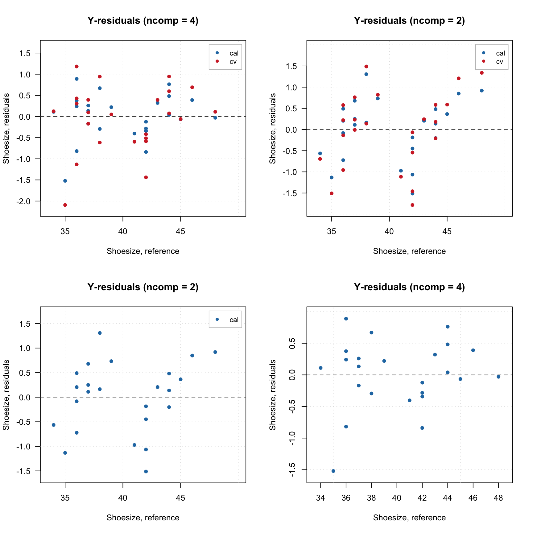
As you can see, all results are very similar to what you got with PV-set, however some of the outcomes (e.g. distances, explained variance, etc) are not available.
In the examples above we set parameter cv to list("ven", 4). But in fact it can be a number, a list or a vector with segment values manually assigned for each measurement.
If it is a number, it will be used as number of segments for random cross-validation, e.g. if cv = 2 cross-validation with two segments will be carried out with measurements being randomly split into the segments. For full cross-validation use cv = 1 like in the example above. This option is a bit confusing, logically we have to set cv equal to the number of measurements in the calibration set. But this option was used many years ago when the package was created and it is kept for backward compatibility.
For more advanced selection you can provide a list with name of cross-validation method, number of segments and number of iterations, e.g. cv = list("rand", 4, 4) for running random cross-validation with four segments and four repetitions or cv = list("ven", 8) for systematic split into eight segments (venetian blinds). In case of venetian splits, the measurements will be automatically ordered from smallest to largest response (y) values.
Finally, you can also provide a vector with manual slits. For example, if you create a model with the following value for cv parameter: cv = rep(1:4, length.out = nrow(Xc)) the vector of values you provide will look as 1 2 3 4 1 2 3 4 1 2 ..., which corresponds to systematic splits but without ordering y-values, so it will use the current order of measurements (rows) in the data. Use this option if you have specific requirements for cross-validation and the implemented methods do not meet them.
Local and global CV scope
From 0.14.1 it is possible to set how cross-validation subsets are centred and scaled inside the cross-validation loop. This is regulated by a new parameter cv.scope in methods pls(), plsda() and ipls().
Cross-validation splits the original training set into local calibration and validation sets inside the loop. For example, if you have dataset with 100 objects/observations and use cross-validation with four segments (with random or systematic splits), in each iteration 25 objects will be taken as local validation set and remaining 75 objects will form a local calibration set.
If cv.scope parameter is set to "local", then mean values for centering and standard deviation values for scaling (if this option is selected) will be computed based on the local set with 75 objects in the example below. So, every local model will have its own center in the variable space.
If cv.scope parameter is set to "global", then the mean values and standard deviation values will be computed for the original (global) training set hence all local models will have the same center as the global model.
The default value is "local" and this was also the way mdatools worked before this option was introduced in 0.14.1. The small example below shows how both options work (it is assumed that you already have Xc and yc variables from the previous examples):
m1 = pls(Xc, yc, 7, cv = list("ven", 4), cv.scope = "local")
m2 = pls(Xc, yc, 7, cv = list("ven", 4), cv.scope = "global")

par(mfrow = c(1, 2))
plotRMSE(m1$res$cv, type = "h", show.labels = TRUE, main = "Local cv-scope")
plotRMSE(m2$res$cv, type = "h", show.labels = TRUE, main = "Global cv-scope")
As you can see, the cross-validation results are very similar, however RMSE values for locally autoscaled models tend to be a bit higher as expected.
Selection of optimal number of components
When you create a PLS model, it tries to select optimal number of components automatically (which, of course, you can always change later). To do that, the method uses RMSE values, calculated for different number of components and validation predictions. So, if we do not use any validation, it warns us about this as it was mentioned in the beginning of this chapter.
If validation (any of the three methods described above) was used, there are two different ways/criteria for automatic selection of the components based on validation results. One is using first local minimum on the RMSE plot and second is so called Wold criterion, based on a ratio between PRESS values for current and next component.
You can select which criterion to use by specifying parameter ncomp.selcrit (either 'min' or 'wold') as it is shown below (here we use cross-validation).
## [1] 3## [1] 3Well, in this case both pointed to the same number, 3, but sometimes they give different solutions.
And here are the RMSE plots (they are identical of course), where you can see how error depends on number of components for both calibration set and cross-validated predictions. Apparently the minimum for cross-validation error (RMSECV) is indeed at 3:
Another useful plot in this case is a plot which shows ratio between cross-validated RMSE values, RMSECV, and the calibrated ones, RMSEC. You can see an example in the figure below and read more about this plot in blog post by Barry M. Wise.