Making predictions
Dataset with target class only
Now let’s check the model performance using independent test set consisting only of the target class members. First of all, we need to load it and split to matrix with predictors and the vector with class labels:
dtt <- read.csv("./Oregano/Target_Test.csv", row.names = 1, check.names = FALSE)

ctt = dtt[, 1]
xtt = as.matrix(dtt[, -1])
And apply the model:
##
## DD-SIMCA results
##
## Target class: Oregano
## Number of components: 10
## Number of selected components: 3
## Type of limits: classic
## Alpha: 0.050
##
## Number of objects: 18
##  - target class members: 18
##  - from non-target classes: 0
##  - from unknown classes: 0
##
##          Expvar Cumexpvar In Out TP FN   Sens
## Comp 1  38.1465     38.15 18   0 18  0 1.0000
## Comp 2  20.4210     58.57 17   1 17  1 0.9444
## Comp 3* 11.5118     70.08 17   1 17  1 0.9444
## Comp 4   9.9178     80.00 14   4 14  4 0.7778
## Comp 5   5.4689     85.47 13   5 13  5 0.7222
## Comp 6   4.6626     90.13 10   8 10  8 0.5556
## Comp 7   5.3661     95.49  8  10  8 10 0.4444
## Comp 8   0.8855     96.38  5  13  5 13 0.2778
## Comp 9   0.3749     96.76  4  14  4 14 0.2222
## Comp 10  1.2238     97.98  4  14  4 14 0.2222
Summary text for result object shows values for all components, but the selected one is marked by * in the table. As one can see, the sensitivity is very similar to the one obtained for PV-set. Let’s compare these two results also with plots:
par(mfrow = c(2, 2))
plotAcceptance(m$res$pv, log = TRUE, show.labels = TRUE)
plotAcceptance(rtt, log = TRUE, show.labels = TRUE)
plotSensitivity(m$res$pv, show.ci = TRUE)
plotSensitivity(rtt, show.ci = TRUE)
Apparently, both PV-set and test set point to \(A = 3\) as optimal selection.
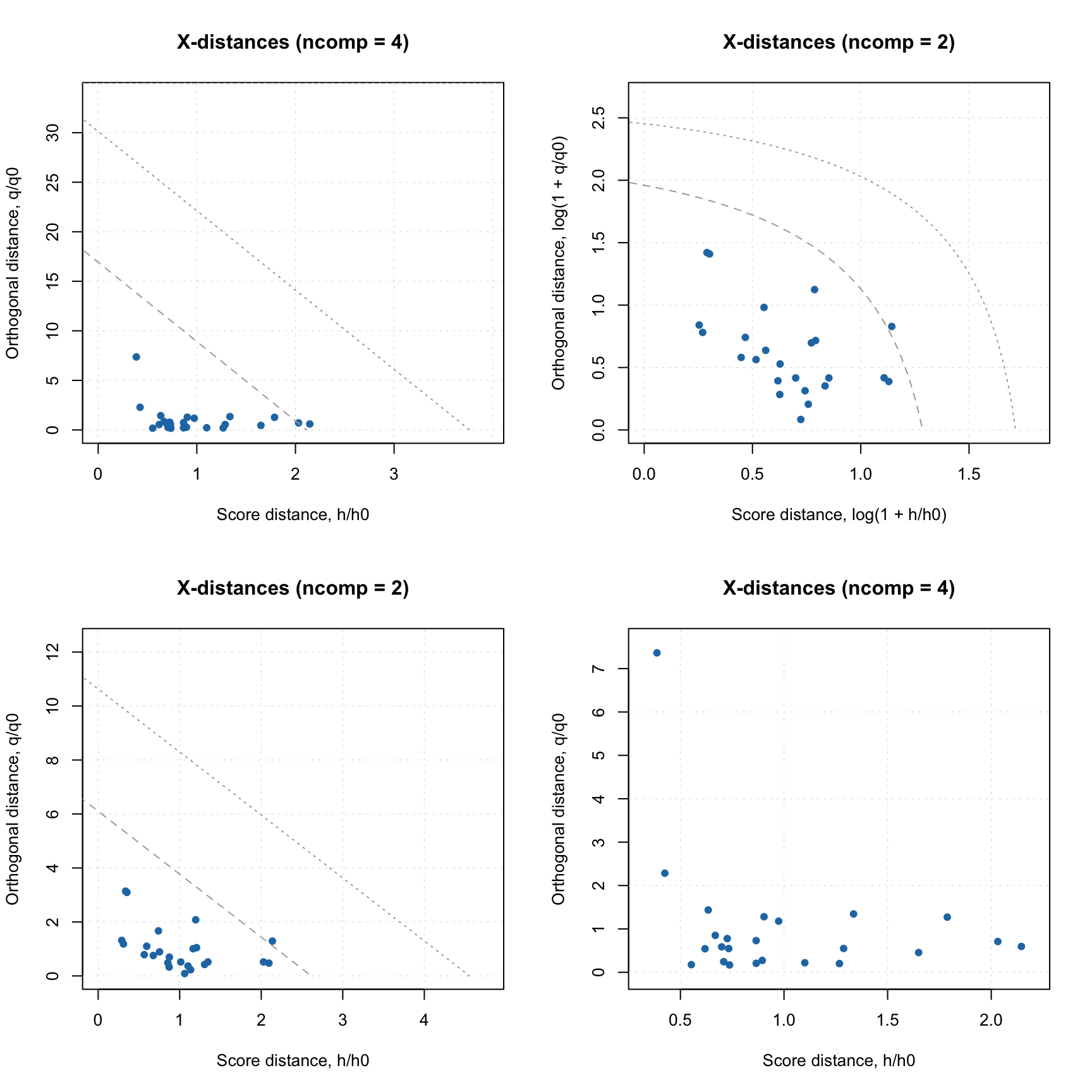
As in case of PCA, one can make Extremes plot for the DD-SIMCA results, which can be helpful in identifying overfitting:

You can get all classification details by converting the DD-SIMCA result object into a data frame:
##         class    role decision      h/h0     q/q0         f
## Dro01 Oregano extreme      out 1.6683669 4.433422 17.208679
## Dro02 Oregano regular       in 0.3595882 1.673141  5.144223
## Dro03 Oregano regular       in 0.6114075 3.530630 10.118297
## Dro04 Oregano regular       in 1.4298180 1.726167 10.601424
## Dro05 Oregano regular       in 0.2364948 2.807929  6.798333
## Dro06 Oregano regular       in 0.3366462 2.794651  7.272534
By default the data frame is created using current model settings. If necessary, you can change this as follows:
##         class    role decision      h/h0     q/q0         f
## Dro01 Oregano extreme      out 0.9142328 4.027964 27.824718
## Dro02 Oregano regular       in 0.5176074 1.110331  8.732413
## Dro03 Oregano regular       in 0.9710622 2.265733 17.478646
## Dro04 Oregano regular       in 0.5654677 2.270967 15.887671
## Dro05 Oregano regular       in 0.3515385 1.817433 12.310749
## Dro06 Oregano regular       in 0.2007634 2.019881 12.922342
This is possible because any DD-SIMCA result object contains outcomes computed for all number of components and both robust and classic estimators for the distance parameters and critical limits. However, if you want to change significance level, you need to change the model first, using method setParams(), and then re-apply the new model to the dataset.
Datasets with objects from alternative classes
Now let’s load data containing non-target class members (spectra of herbs, which are not Oregano). This dataset is organized a bit differently, the row names are located in a dedicated column, plus some of the row names are not unique, therefore we use a bit modified procedure:
dtn = read.csv("./Oregano/NonTarget_Non_Or.csv", check.names = FALSE)

# get rownames and make them unique
objnames = dtn[, 1]
objnames = paste0(objnames, ".", seq_along(objnames))

ctn = dtn[, 2]
xtn = as.matrix(dtn[, -c(1, 2)])
rownames(xtn) = objnames
And apply the model:
##
## DD-SIMCA results
##
## Target class: Oregano
## Number of components: 10
## Number of selected components: 3
## Type of limits: classic
## Alpha: 0.050
##
## Number of objects: 49
##  - target class members: 0
##  - from non-target classes: 49
##  - from unknown classes: 0
##
##          Expvar Cumexpvar In Out TN FP  Spec    Sel
## Comp 1  17.0005     17.00  5  44 44  5 0.898 0.8997
## Comp 2  35.5382     52.54  0  49 49  0 1.000 0.9692
## Comp 3* 29.5319     82.07  0  49 49  0 1.000 0.9682
## Comp 4   3.6730     85.74  0  49 49  0 1.000 0.9835
## Comp 5   2.1846     87.93  0  49 49  0 1.000 0.9894
## Comp 6   6.4556     94.38  0  49 49  0 1.000 0.9840
## Comp 7   1.3279     95.71  0  49 49  0 1.000 0.9948
## Comp 8   1.6068     97.32  0  49 49  0 1.000 0.9943
## Comp 9   0.2181     97.54  0  49 49  0 1.000 0.9988
## Comp 10  0.5038     98.04  0  49 49  0 1.000 0.9997
Now you can spot the difference. First of all, because this dataset does not contain any target class members, the table does not have columns for true positives (TP), false negatives (FN) and sensitivity. In contrast, it has columns for true negatives (TN), false positives (FP), as well as selectivity and specificity.
Therefore the Acceptance plot also looks different:
par(mfrow = c(1, 2))
plotAcceptance(rtn, show.labels = TRUE)
plotAcceptance(rtn, log = TRUE, show.labels = TRUE)
In this case we know in advance that all objects are from non-target classes, so they are supposed to be extreme. But they are extreme in a different way. The ones marked with role “alien” are objects from possibly the same population, closest to the target class. The objects marked as “external” are possibly from other groups/populations which are the most distinct from the target class. The plot also does not contain the limits for outliers, as “outlier” is a role that can be assigned only to a target class member.
The specificity is computed based on all non-target class objects. While selectivity is computed only by taking the “aliens” into account. Moreover, in this case we fit aliens with non-central chi-square distribution and find the overlap between the distribution of the target class objects and the distribution of the aliens. The selectivity is related to this overlap.
This approach is also known as power of test in statistics. It gives more realistic estimate on how the model will behave for rejecting the aliens. The value complementary to selectivity is a chance of making Type II error, \(\beta\). For example for \(A = 3\) the beta is \(1 - 0.9682 = 0.0318\) or approximately 3%.
The selectivity can be visualized as ROC curve, showing changes in selectivity values depending on significance level used in the model:
The plot shows the dependence as a curve and the current model as a point on the curve. It also computes the area under the curve (AUC), which can be used as auxiliary figure of merit.
Datasets with objects from both target and alternative classes
One can also apply DD-SIMCA model to a dataset containing both target and non-target class members. In this case one can use a compliance approach for finding optimal number of components. Let’s load the data first:
dta = read.csv("./Oregano/All_Test.csv", check.names = FALSE)

objnames = dta[, 1]
cta = dta[, 2]
xta = as.matrix(dta[, -c(1, 2)])
rownames(xta) = objnames
And apply the model
##
## DD-SIMCA results
##
## Target class: Oregano
## Number of components: 10
## Number of selected components: 3
## Type of limits: classic
## Alpha: 0.050
##
## Number of objects: 67
##  - target class members: 18
##  - from non-target classes: 49
##  - from unknown classes: 0
##
##          Expvar Cumexpvar In Out TP FN   Sens TN FP  Spec    Sel    Acc    Eff
## Comp 1  17.9265     17.93 23  44 18  0 1.0000 44  5 0.898 0.8997 0.9254 0.9476
## Comp 2  34.8762     52.80 17  50 17  1 0.9444 49  0 1.000 0.9692 0.9851 0.9718
## Comp 3* 28.7428     81.55 17  50 17  1 0.9444 49  0 1.000 0.9682 0.9851 0.9718
## Comp 4   3.9465     85.49 14  53 14  4 0.7778 49  0 1.000 0.9835 0.9403 0.8819
## Comp 5   2.3285     87.82 13  54 13  5 0.7222 49  0 1.000 0.9894 0.9254 0.8498
## Comp 6   6.3771     94.20 10  57 10  8 0.5556 49  0 1.000 0.9840 0.8806 0.7454
## Comp 7   1.5047     95.70  8  59  8 10 0.4444 49  0 1.000 0.9948 0.8507 0.6667
## Comp 8   1.5752     97.28  5  62  5 13 0.2778 49  0 1.000 0.9943 0.8060 0.5270
## Comp 9   0.2250     97.50  4  63  4 14 0.2222 49  0 1.000 0.9988 0.7910 0.4714
## Comp 10  0.5353     98.04  4  63  4 14 0.2222 49  0 1.000 0.9997 0.7910 0.4714
As you can see the summary table in this case is much larger containing all outcomes and figures of merit. In addition to sensitivity, specificity and selectivity, it also has columns for efficiency (the geometric mean of the two) and accuracy.
All these figures of merit can be visualized individually or all together. Here are some examples:
par(mfrow = c(2, 2))
plotFoM(rta, fom = "sens")
plotFoM(rta, fom = "eff")
plotFoMs(rta, fom = c("sens", "spec", "eff"))
plotFoMs(rta, fom = c("spec", "sel"), legend.position = "bottomright",
pch = c(16, 4), col = c("blue", "red"))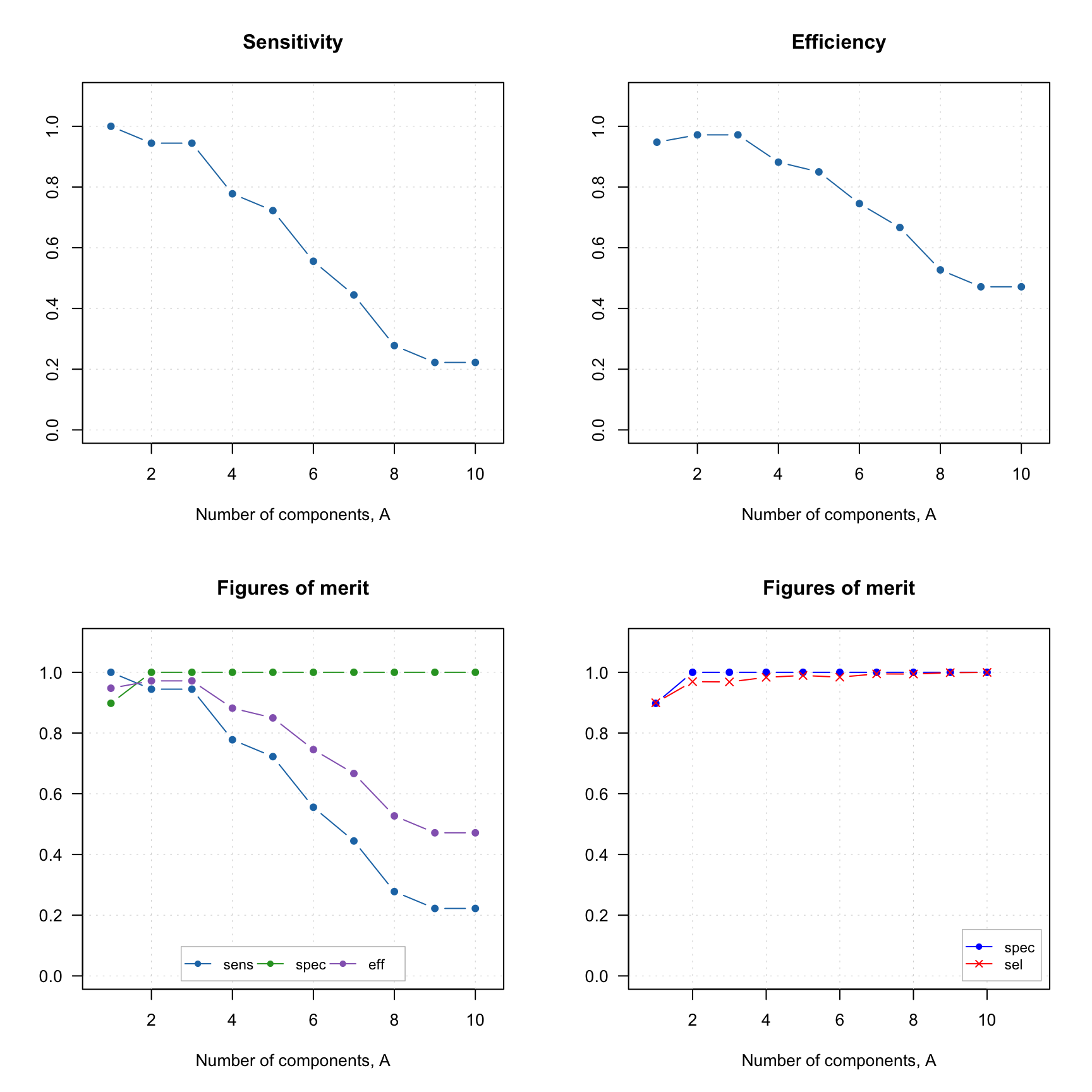 And of course similar to other plots one can define own colors, markers, etc.
When you make Acceptance plot, you need to specify, whether you want to show only members (this is a default option), only strangers or both. In the latter case the objects will be color grouped by the reference classes:
par(mfrow = c(2, 2))
plotAcceptance(rta)
plotAcceptance(rta, show = "members")
plotAcceptance(rta, show = "strangers", log = TRUE)
plotAcceptance(rta, show = "all", log = TRUE)
Datasets without reference classes
If no reference class labels are provided, the objects are considered as unknown (new) and no FoMs are computed. In this case only acceptance and distance plots are available (as well as all PCA plots of course). Let’s use the non-target class data again (I assume you have it loaded), but we will not provide the vector with reference classes this time:
##
## DD-SIMCA results
##
## Target class: Oregano
## Number of components: 10
## Number of selected components: 3
## Type of limits: classic
## Alpha: 0.050
##
## Number of objects: 49
##  - target class members: 0
##  - from non-target classes: 0
##  - from unknown classes: 49
##
##          Expvar Cumexpvar In Out
## Comp 1  17.0005     17.00  5  44
## Comp 2  35.5382     52.54  0  49
## Comp 3* 29.5319     82.07  0  49
## Comp 4   3.6730     85.74  0  49
## Comp 5   2.1846     87.93  0  49
## Comp 6   6.4556     94.38  0  49
## Comp 7   1.3279     95.71  0  49
## Comp 8   1.6068     97.32  0  49
## Comp 9   0.2181     97.54  0  49
## Comp 10  0.5038     98.04  0  49
And here is how the data frame with outcomes looks like:
##         decision      h/h0      q/q0         f
## Bas01.1      out 11.580328  6.034440  69.97052
## Bas02.2      out 13.022050 12.767634  90.64552
## Bas03.3      out  8.137095 14.658761  70.00300
## Cel01.4      out 34.464145 11.237176 194.79508
## Cel02.5      out 32.563306  8.966258 180.74904
## Cel03.6      out 31.860073  9.742277 178.78492
It does not contain column “roles” anymore, only the decision (“in” or “out”).
If you try to make a plot with figures of merit, you will get an error, as none of them can be found. But Acceptance plot still works of course: