Interoperability with web-application
Similar to PCA and preprocessing there is an interactive web-application, https://mda.tools/ddsimca, which lets you create DD-SIMCA models and apply them to a new dataset in any modern browser. Any DD-SIMCA model created using ddsimca() can be saved into a JSON file and then be loaded into the Project tab of the web-application. Including preprocessing methods.
Here is an example based on the model created in the previous section (let’s repeat this code again here, just in case):
p = list(
   prep("savgol", width = 9, porder = 1, dorder = 1),
   prep("norm", type = "snv")
)

m = ddsimca(xc, "Oregano", ncomp = 10, pcv = list("ven", 4), prep = p, exclrows = c("Drg12", "Drg13"))
m = selectCompNum(m, 3)

# save the model to JSON file
writeJSON(m, "ddsimca-model.json")
If you run the code on your computer you will see a new ddsimca-model.json file created in the working directory. Now open https://mda.tools/ddsimca in your browser, select tab Test and load the file with the model. You will see something similar to the following:
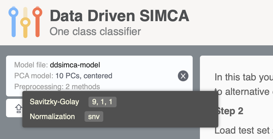
After that you can upload any CSV file we used in this chapter and see the result of classification directly in the app.
Likewise, any DD-SIMCA model created in the application can be saved into a JSON file and loaded into R, so you can use it via predict(). For example this JSON file I created using the same Oregano training set but it has no preprocessing, \(A = 2\) as the optimal number of components, and significance levels \(\alpha = 0.01\), \(\gamma = 0.001\).
Download it to your working directory and run the following code (here I assume you already have xta matrix and corresponding cta vector from the previous blocks of code):
# load PCA model from JSON file
m <- readJSON("ddsimca-model-fromweb.json")

# apply it to test set with all objects
r <- predict(m, xta, cta)
summary(r)
##
## DD-SIMCA results
##
## Target class: Oregano
## Number of components: 20
## Number of selected components: 2
## Type of limits: classic
## Alpha: 0.010
##
## Number of objects: 67
## - target class members: 18
## - from non-target classes: 49
## - from unknown classes: 0
##
## Expvar Cumexpvar In Out TP FN Sens TN FP Spec Sel Acc
## Comp 1 17.92650 17.93 30 37 18 0 1.0000 37 12 0.7551 0.8155 0.8209
## Comp 2* 34.87615 52.80 20 47 18 0 1.0000 47 2 0.9592 0.9347 0.9701
## Comp 3 28.74276 81.55 20 47 18 0 1.0000 47 2 0.9592 0.9350 0.9701
## Comp 4 3.94647 85.49 16 51 16 2 0.8889 49 0 1.0000 0.9621 0.9701
## Comp 5 2.32847 87.82 15 52 15 3 0.8333 49 0 1.0000 0.9755 0.9552
## Comp 6 6.37712 94.20 13 54 13 5 0.7222 49 0 1.0000 0.9638 0.9254
## Comp 7 1.50471 95.70 12 55 12 6 0.6667 49 0 1.0000 0.9858 0.9104
## Comp 8 1.57521 97.28 10 57 10 8 0.5556 49 0 1.0000 0.9845 0.8806
## Comp 9 0.22496 97.50 6 61 6 12 0.3333 49 0 1.0000 0.9960 0.8209
## Comp 10 0.53530 98.04 6 61 6 12 0.3333 49 0 1.0000 0.9990 0.8209
## Comp 11 0.12531 98.16 5 62 5 13 0.2778 49 0 1.0000 0.9997 0.8060
## Comp 12 0.06786 98.23 5 62 5 13 0.2778 49 0 1.0000 0.9999 0.8060
## Comp 13 0.09338 98.32 2 65 2 16 0.1111 49 0 1.0000 1.0000 0.7612
## Comp 14 0.07814 98.40 0 67 0 18 0.0000 49 0 1.0000 1.0000 0.0000
## Comp 15 0.07341 98.48 0 67 0 18 0.0000 49 0 1.0000 1.0000 0.0000
## Comp 16 0.12804 98.60 0 67 0 18 0.0000 49 0 1.0000 1.0000 0.0000
## Comp 17 0.03662 98.64 0 67 0 18 0.0000 49 0 1.0000 1.0000 0.0000
## Comp 18 0.09743 98.74 0 67 0 18 0.0000 49 0 1.0000 1.0000 0.0000
## Comp 19 0.07831 98.82 0 67 0 18 0.0000 49 0 1.0000 1.0000 0.0000
## Comp 20 0.13056 98.95 0 67 0 18 0.0000 49 0 1.0000 1.0000 0.0000
## Eff
## Comp 1 0.8690
## Comp 2* 0.9794
## Comp 3 0.9794
## Comp 4 0.9428
## Comp 5 0.9129
## Comp 6 0.8498
## Comp 7 0.8165
## Comp 8 0.7454
## Comp 9 0.5774
## Comp 10 0.5774
## Comp 11 0.5270
## Comp 12 0.5270
## Comp 13 0.3333
## Comp 14 0.0000
## Comp 15 0.0000
## Comp 16 0.0000
## Comp 17 0.0000
## Comp 18 0.0000
## Comp 19 0.0000
## Comp 20 0.0000par(mfrow = c(1, 2))
plotFoMs(r, fom = c("sens", "spec", "eff"), legend.position = "bottomleft")
plotAcceptance(r, show = "all", log = TRUE)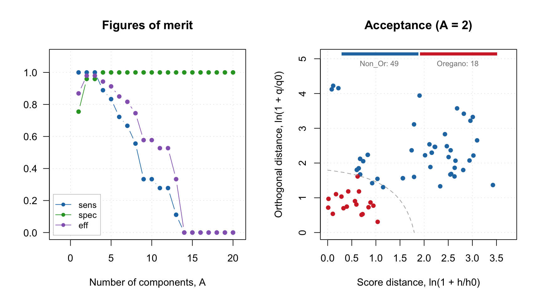
There is also a limitation though, model loaded from JSON file created by the web-application does not contain calibration results, it can only be used for predictions/projections:
##
## DD-SIMCA model for class 'Oregano'
##
## Number of components: 20
## Number of selected components: 2
## Type of limits: robust
## Alpha: 0.01
## Gamma: 0.001
## Calibration results not found (most probably this model is loaded from web-application).Most of the plots, which rely on calibration set results will not work with such model object and give you the same message as above. However plots, which are only based on model outcomes, such as loadings, eigenvalues and degrees of freedom are available: