Interoperability with web-applications
Similar to preprocessing there is an interactive web-application, https://mda.tools/pls, which lets you create PLS models and apply them to a new dataset in any modern browser. Any PLS model created using pls() can be saved into a JSON file and then be loaded into the Project tab of the web-application. Including preprocessing methods!
Here is an example based on Simdata:
# define calibration set
Xc = simdata$spectra.c
yc = simdata$conc.c[, 2, drop = FALSE]

# create a sequence of preprocessing methods
p <- list(
   prep("savgol", width = 11, porder = 2, dorder = 2),
   prep("varsel", var.ind = 20:120)
)

# create a PCA model with preprocessing as a part of the model
m <- pls(Xc, yc, 6, prep = p)
## Warning in selectCompNum.pls(model, selcrit = ncomp.selcrit): No validation
## results were found.If you run the code on your computer you will see a new pls-model.json file created in the working directory. Now open https://mda.tools/pls in your browser, select tab Project and load the file with the model. You will see something similar to the following:
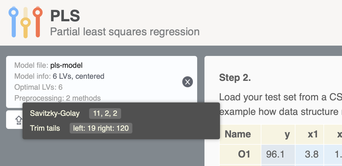
After that you can upload dataset and see the result of projecting it to the PLS model directly in the app.
Likewise, any PLS model created in the application can be saved into a JSON file and loaded into R, so you can use it via predict(). For example this JSON file I created using the Train tab of the app and Simdata. It contains a PLS model on data with a preprocessing chain that includes SG smoothing with first derivative, trimming tails, and mean centering. Download it to your working directory and run the following code (here I assume you already have Xc and yc matrices from the previous blocks of code):
# load preprocessing model from JSON file
m <- readJSON("pls-model-fromweb.json")

# apply it to Xc
r <- predict(m, Xc, yc)
summary(r)
##
## PLS regression results (class plsres) summary
## Info:
## Number of selected components: 2
##
## Response variable C2:
## X expvar X cumexpvar Y expvar Y cumexpvar R2 RMSE Slope Bias RPD
## Comp 1 97.380 97.380 13.844 13.844 0.138 0.138 0.138 0 1.08
## Comp 2 2.217 99.597 82.714 96.557 0.966 0.028 0.966 0 5.42
## Comp 3 0.326 99.923 0.052 96.609 0.966 0.027 0.966 0 5.46
## Comp 4 0.005 99.928 0.727 97.336 0.973 0.024 0.973 0 6.16
## Comp 5 0.003 99.931 0.464 97.799 0.978 0.022 0.978 0 6.78
## Comp 6 0.003 99.934 0.372 98.172 0.982 0.020 0.982 0 7.43
## Comp 7 0.003 99.937 0.190 98.362 0.984 0.019 0.984 0 7.85
## Comp 8 0.003 99.940 0.163 98.525 0.985 0.018 0.985 0 8.27
## Comp 9 0.003 99.943 0.124 98.648 0.986 0.017 0.986 0 8.64
## Comp 10 0.002 99.945 0.171 98.819 0.988 0.016 0.988 0 9.25
## Comp 11 0.002 99.947 0.141 98.960 0.990 0.015 0.990 0 9.86
## Comp 12 0.003 99.950 0.109 99.069 0.991 0.014 0.991 0 10.42
There is also a limitation though, model loaded from JSON file created by the web-application does not contain calibration results, it can only be used for predictions:
##
## PLS model (class pls) summary
## -------------------------------
## Info:
## Number of selected components: 2
## Cross-validation: none
##
## Preprocessing methods:
##  - savgol: width = 9, porder = 1, dorder = 1
##  - varsel: var.ind = 13:132
## Objects with results not found (most probably this model is loaded from web-application).Most of the plots, which rely on calibration set results will not work with such model object and give you the same message as above. However plots, which are only based on model outcomes, such as loadings, weights and regression coefficients are available: